SAM from Meta AI (Part 1): Segmentation with Prompts

---

Table of Contents

---

SAM from Meta AI (Part 1): Segmentation with Prompts

In this tutorial, you will learn about the Segment Anything Model (SAM) from Meta AI and delve deeper into the ideas and concepts behind this newly released foundational segmentation model. Furthermore, you will learn how SAM can be used for making segmentation predictions in real-time and how you can integrate it with your own computer vision projects.

This lesson is the 1st of a 2-part series on Segment Anything Model (SAM) from Meta AI:

1. SAM from Meta AI (Part 1): Segmentation with Prompts (this tutorial)
2. SAM from Meta AI (Part 2): Integration with CLIP for Downstream Tasks

In the first part of this tutorial series, we will develop a holistic understanding of SAM and discuss in detail how SAM can be prompted in different ways, which allows it to segment specific regions in any image in real-time.

In the second part of this tutorial, we will take a step ahead and understand how SAM can be integrated with other foundational models like contrastive language-image pre-training (CLIP) to perform varied downstream tasks like zero-shot classification, text-to-image retrieval, and image similarity.

To learn how to use SAM in your own projects, just keep reading.

---

SAM from Meta AI (Part 1): Segmentation with Prompts

In the past, computer vision models have mostly relied on methods trained on a specific task with task-specific annotated datasets. They can perform that particular task on novel examples at test time. This affects the practical usability of these models since it is not always possible or feasible to have access to or collect large amounts of data for every task at hand.

Furthermore, the generalization performance of these models considerably deteriorates if the distribution of examples at test time deviates from the data distribution of the training examples. This limited their applicability in practical, real-world applications where we need systems that can perform multiple downstream tasks effectively and are robust to distribution shifts.

To address the aforementioned issues, there has been considerable effort in the computer vision community to develop models with more general capabilities that can holistically understand data and perform various downstream tasks of varied data distributions.

Recent progress toward developing such general-purpose “foundational models” has boomed the machine learning and computer vision community. This direction of research was first explored by the natural language processing (NLP) community (which eventually led to the development of ChatGPT) and has gradually been picked up by the computer vision folks to develop holistic general-purpose models which can perform varied tasks alone or can be integrated into pre-established systems to improve performance.

In computer vision, the recent foundational models mainly rely on utilizing large scale web-data and aligning image and text pairs to train strong representation models. One such example is the CLIP model, which learns representations that understand the semantics of various objects and can generalize them in a zero-shot way (i.e., without further fine-tuning). The CLIP model shows exceptional results on zero-shot image classification tasks and can outperform various fine-tuned supervised models.

Along similar lines, Meta AI recently released the segment anything model (SAM), the first attempt to design a foundational model for image segmentation. SAM can perform segmentation on data from various distributions and can adapt to solve several downstream tasks at test time. Furthermore, SAM can be seamlessly integrated with pre-established computer vision models and systems to boost their capabilities and performance on complex tasks for which training task-specific models would not be feasible.

---

Segment Anything

The SAM marks the first step toward developing general-purpose foundational models for image segmentation tasks. Like other foundational models, it is pre-trained on a large-scale dataset with 11 million images annotated with 1 billion masks. This allows it to generalize to diverse image distributions and objects at test time (https://segment-anything.com/dataset/index.html).

SAM is designed and developed to be promptable, allowing it to seamlessly tackle different tasks at inference, including those it was not trained to perform. Furthermore, this will enable it to seamlessly integrate with other computer vision systems for different downstream tasks apart from image segmentation. Let us discuss this in further detail to understand the key ideas behind this approach.

Prompt engineering refers to crafting text inputs to get desired responses from foundational models. For example, engineered text prompts are used to query ChatGPT and get a useful or desirable response for the user. CLIP is prompted with hand-engineered text prompts to enhance its zero-shot classification performance on object categories, etc.

Using the aforementioned foundational models, SAM designs a promptable segmentation task with a prompt in the form of a point, bounding box, or text. The model tries to predict a segmentation mask for the region indicated by the input prompt. Once the model is trained, SAM can be prompted with various engineered prompts per the downstream task to enable a wide range of downstream applications similar to other foundational models like ChatGPT and CLIP.

Let us delve deeper and get an overview of the training and inference details, which allow SAM to generalize to new data distributions and tasks at inference.

---

Training SAM

SAM is pre-trained with a prompt-based segmentation pre-training objective. Specifically, it involves a sequence of prompts (e.g., points, boxes, masks) input to the model with an image sample. The model outputs a segmentation mask prediction based on the prompt, which is then compared with the ground truth segmentation mask to compute the loss.

Figure 1 shows an overview of the SAM training pipeline. First, an image is input to the transformer-based image encoder, which outputs feature representation as image embeddings, as shown in the figure. SAM uses a masked autoencoder-based pre-trained vision transformer as the image encoder.

Next, the model takes input prompts such as points, bounding boxes, text, or masks and encodes them using the prompt encoder and convolutions (shown in purple).

The mask decoder (shown in yellow) maps the input representations of the image and the prompts to an output mask which is then compared with the ground truth mask to compute the loss and backpropagate through the network.

SAM uses focal loss and dice loss for training the model. The focal loss is simply a variation of the cross-entropy loss function, ensuring that the pixels are classified correctly in the predicted segmentation mask. On the other hand, the dice loss aims to increase the overlap (i.e., the intersection over the union area, to be more precise) between the predicted and ground truth mask.

---

Inference with SAM

Once SAM is pre-trained with the promptable segmentation objective mentioned above, it can be used to segment objects or regions in images based on the input prompt provided by the user.

For example, given an image of a kitchen with a potted plant on the slab, we can sample single or multiple points on the plant region and pass them as input to SAM to segment out the plant in the image. We can also provide a bounding box around the potted plant and ask SAM to segment the object inside the bounding box.

Furthermore, we can also use prompting to specify further and control the region we want segmented. For instance, if we want to segment only the region with plant branches and leaves and exclude the pot which holds the plant, we can simply pass points on the plant region as positive points and the points on the potted region as negative points. This indicates to the model to predict a segmentation mask for the region, which includes the positive points and excludes the negative points.

Additionally, we can use any combination of these prompts to specify the region where we want to segment the object. For instance, we can provide a combination of bounding box coordinates and negative points to specify a region inside the box but exclude the negative point.

Note that currently, the released code for SAM does not directly support text-based prompts. However, in this tutorial, we will see how to integrate SAM with another off-the-shelf model (i.e., Grounding DINO) to use text prompts for segmenting objects.

Let us now go ahead and implement the code to perform segmentation tasks as explained above and see our SAM make predictions in real-time.

---

Project Structure

We first need to review our project directory structure.

Start by accessing this tutorial’s “Downloads” section to retrieve the source code and example images.

From there, take a look at the directory structure:

├── clip_integration.py
├── gdino_integration.py
├── get_objects.py
├── images
│   ├── kitchen.jpeg
│   └── living_room.jpg
├── pyimagesearch
│   ├── config.py
│   └── utils.py
├── requirements.txt
├── sam.py
└── setup.sh

We first have the checkpoints folder, which contains the pre-trained checkpoints for SAM and the Grounding DINO model, as we will see later in this tutorial.

The clip_integration.py file implements the code to integrate SAM with CLIP, which we will discuss in depth in the next tutorial of this series.

Furthermore, the gdino_integration.py file implements the code, allowing us to prompt SAM with text prompts with the help of Grounding DINO and predict segmentation masks in real-time.

Next, in the directory structure, we have the get_objects.py file, which we will discuss in detail in the next tutorial in this series, and the images folder, which consists of the two images we will use for this tutorial series.

In the pyimagesearch folder, we have the config.py and utils.py files, which define the parameters, initial configurations, and helper functions, allowing us to visualize our predictions, respectively.

Furthermore, the sam.py file implements the code to use different prompts like points and bounding boxes to predict segmentation masks with SAM.

Finally, the requirements.txt file contains the required packages and modules to set up our environment and the setup.sh file contains code to download other dependencies and pre-trained checkpoints

---

Configuring Your Development Environment

To follow this guide, you need to have the SAM and off-the-shelf Grounding DINO packages installed. Furthermore, you will need to download the pre-trained checkpoints for these models.

Luckily, this can be done easily by following the commands below:

$ sh setup.sh
$ pip install -r requirements.txt

---

Need Help Configuring Your Development Environment?

All that said, are you:

• Short on time?
• Learning on your employer’s administratively locked system?
• Wanting to skip the hassle of fighting with the command line, package managers, and virtual environments?
• Ready to run the code immediately on your Windows, macOS, or Linux system?

Then join PyImageSearch University today!

Gain access to Jupyter Notebooks for this tutorial and other PyImageSearch guides pre-configured to run on Google Colab’s ecosystem right in your web browser! No installation required.

And best of all, these Jupyter Notebooks will run on Windows, macOS, and Linux!

---

Creating Our Configuration File

It is now time to start our implementation and see some code in action which allows us to segment objects with prompts in real-time.

We start by opening our config.py file, which contains the initial parameters and configurations we will use in this tutorial.

SAM_CHECKPOINT_PATH = "checkpoints/sam_vit_h_4b8939.pth"
MODEL_TYPE = "vit_h"

GDINO_CONFIG = "GroundingDINO/groundingdino/config/GroundingDINO_SwinT_OGC.py"
GDINO_CHECKPOINT_PATH = "checkpoints/groundingdino_swint_ogc.pth"

IMG_PATH = ["images/kitchen.jpeg", "images/living_room.jpg"]
TEXT_PROMPT = ["plant", "apples", "vase"]
IMG_SIZE = (256, 256)

BOX_TRESHOLD = 0.35
TEXT_TRESHOLD = 0.25

OUT_PATH = "predictions"
OUT_PROMPT_PATH = "prompt_image.jpg"
OUT_PRED_PATH = "predicted_image.jpg"

We start defining the SAM_CHECKPOINT_PATH, which points to the location where pre-trained weights of SAM will store (Line 1), and also define the MODEL_TYPE, which indicates the type of vision transformer architecture to use for the image encoder in the SAM architecture (Line 2).

Next, we define the path to the configuration file (i.e., GDINO_CONFIG) for the Grounding DINO model on Line 4, which will help us get segmentations for text prompts from SAM, as we will discuss later in the tutorial. Furthermore, we also define the path to the pre-trained Grounding DINO checkpoint on Line 5 (i.e., GDINO_CHECKPOINT_PATH).

Now that we have defined the model-related parameters, let us go ahead and define the image and prompt-related parameters next.

On Line 7, we define the paths to the two images we will use for the purpose of this tutorial as a list (i.e., IMG_PATH). Next, on Line 8, we define the list TEXT_PROMPT, which contains the various text-based prompts we will use to query our model for segmentation prediction. On Line 9, we define the IMG_SIZE, which indicates the dimension of the images.

Apart from this, we also define the thresholds for bounding box and text (i.e., BOX_TRESHOLD and TEXT_TRESHOLD) on Lines 11 and 12, which the Grounding DINO model will use to make predictions as well and which we will discuss in detail later in the tutorial.

Finally, we define the parameters for the output folder where our predictions will be stored.

On Line 14, we define the OUT_PATH, which points to the folder’s location where our predictions will be stored. Furthermore, on Lines 15 and 16, we define the filenames that will be used to save our image with the prompt visualization (i.e., OUT_PROMPT_PATH) and the final image with the predicted segmentation (i.e., OUT_PRED_PATH).

---

Implementing Visualization Functions

Now that we have discussed the parameter configurations, let us implement and discuss the helper functions, allowing us to visualize our prompt and final segmentation predictions from SAM.

We open the utils.py file and get started.

import matplotlib.pyplot as plt
import numpy as np


def show_points(coords, labels, ax, marker_size=375):
    pos_points = coords[labels == 1]
    neg_points = coords[labels == 0]
    ax.scatter(
        pos_points[:, 0],
        pos_points[:, 1],
        color="green",
        marker="*",
        s=marker_size,
        edgecolor="white",
        linewidth=1.25,
    )
    ax.scatter(
        neg_points[:, 0],
        neg_points[:, 1],
        color="red",
        marker="*",
        s=marker_size,
        edgecolor="white",
        linewidth=1.25,
    )


def show_box(box, ax, processed_dim=False):
    x0, y0 = box[0], box[1]
    if processed_dim:
        w, h = box[2], box[3]
    else:
        w, h = box[2] - box[0], box[3] - box[1]
    ax.add_patch(
        plt.Rectangle((x0, y0), w, h, edgecolor="green", facecolor=(0, 0, 0, 0), lw=2)
    )


def show_mask(mask, ax):
    color = np.array([0, 0, 1, 0.6])
    h, w = mask.shape[-2:]
    mask_image = mask.reshape(h, w, 1) * color.reshape(1, 1, -1)
    ax.imshow(mask_image)


def show_all_masks(masks):
    sorted_masks = sorted(masks, key=(lambda x: x["area"]), reverse=True)
    ax = plt.gca()
    ax.set_autoscale_on(False)

    img = np.ones(
        (
            sorted_masks[0]["segmentation"].shape[0],
            sorted_masks[0]["segmentation"].shape[1],
            4,
        )
    )
    img[:, :, 3] = 0
    for mask in sorted_masks:
        m = mask["segmentation"]
        color_mask = np.concatenate([np.random.random(3), [0.35]])
        img[m] = color_mask
    ax.imshow(img)

We start by importing the necessary packages, such as matplotlib (Line 1) and numpy (Line 2).

Next, we define our helper functions which will allow us to plot the different prompts and visualize the segmentation masks.

We start by implementing the show_points function (Lines 5-25), which allows us to visualize the points in the prompt by plotting them on the figure input to the function.

The function takes as input the point coordinates, binary labels corresponding to the points (indicating whether we want the region with or without the point in the predicted segmentation mask), the matplotlib figure parameter (i.e., ax), and the marker_size for the plotted point (Line 5).

Next, we get the points with labels equal to 1, store them as pos_points, and also get the points with labels equal to 0 and store them as neg_points (Lines 6 and 7).

Then we use the matplotlib scatter() function to plot the pos_points with green color and the neg_points with red color, as shown on Lines 8-25. Note that this function takes as input the x and y coordinates of the points, the marker type, the color for the marker to plot, the size of the marker, the color of the edge, and the width of line as shown.

Next, we define the show_box function, which allows us to visualize the bounding box in the prompt by plotting it on the figure input to the function.

The function takes as input the box (i.e., a list with coordinates of the box), the matplotlib figure parameter (i.e., ax) on which we want to plot the box and the processed_dim argument.

Note that the input box provided as argument (which is a set of 4 values) can be in either of 2 formats, that is,

• Case 1: x, y coordinates of bottom left corner and x, y coordinates of the top right corner
• Case 2: x, y coordinates of bottom left corner and the width and height of the box.

The processed_dim argument states which format the bounding box is provided in. It is False in Case 1 and True in Case 2.

On Line 29, we get the x0, y0 coordinates as shown. In case the processed_dim flag is True, we get the width and height of the bounding box (i.e., box[2] and box[3]), as shown on Line 31. If not, we compute the width and height of the bounding box as follows, w=box[2]-box[0] and h=box[3]-box[1]), as shown on line Line 33.

Finally, we use the add_patch function from matplotlib and plot a green-colored rectangle using the plt.Rectangle function, as shown on Lines 34-36.

Now that we have implemented functions to visualize the prompts, we define the functions that will allow us to visualize the segmentation masks.

We start with the show_mask function, which takes as input a single predicted mask, the matplotlib figure parameter (i.e., ax) on which we want to plot and visualize the mask.

On Line 40, we define the color, which is an array with the R, G, B value and the value of transparency with which the mask is plotted on the image (i.e., [0, 0, 1, 0.6]). Next, we get the height and width of the input mask (Line 41).

Next, we reshape the mask to have the shape in the format (h,w,1), reshape the color to have shape (1,1,4), and multiply both, as shown on Line 42. This broadcasts the mask to the shape (h,w,4) and color to the shape (h,w,4), which gets multiplied elementwise.

We finally use the imshow() function to visualize the mask_image, as shown on Line 43.

We now define a function to visualize multiple masks together, which we will use in the next tutorial of this series.

The show_all_masks function (Lines 46-63) takes as input the masks, as shown on Line 46.

On Line 47, we sort the input masks in decreasing order of their area and store them in sorted_masks. Next, we initialize the matplotlib figure on Lines 48 and 49.

On Line 51, we initialize an array of ones of the shape with height=sorted_masks[0]['segmentation'].shape[0], width=sorted_masks[0]['segmentation'].shape[1], and channels=4. Furthermore, we set the third dimension of this array to 0, as shown on Line 58.

Next, for each mask in the sorted_masks list (Line 59), we get the corresponding segmentation mask (Line 60) and create a color_mask with random R, G, and B values with 0.35 as the transparency value (Line 61). We assign the color mask shown on Line 62 to plot the predicted segmentation mask with the color_mask.

Finally, on Line 63, we show the final image using matplotlib.

---

Segmentation with SAM

Now that the implementation of configurations and helper function is complete, we are ready to dive deeper into the code, which allows us to use SAM and make segmentation predictions.

Specifically, we will use prompts such as point coordinates or bounding box coordinates to segment objects of interest in real-time, as discussed above.

Let us open the sam.py file and get started.

# USAGE
# python sam.py

# import the necessary packages
from pyimagesearch import config, utils
from segment_anything import SamPredictor, sam_model_registry
import matplotlib.pyplot as plt
import numpy as np
import cv2
import os

# function to visualize and save segmentation
def visualize_and_save_segmentation(
    prompt, model, query_index, save_multiple_masks=False
):
    input_points, input_labels, input_box = prompt

    # Create output directory if it doesn't exist
    if not os.path.exists(config.OUT_PATH):
        os.makedirs(config.OUT_PATH)

    # Define paths to save prompt and prediction images
    prompt_path = os.path.join(
        config.OUT_PATH, f"{query_index}-{config.OUT_PROMPT_PATH}"
    )
    prediction_path = os.path.join(
        config.OUT_PATH, f"{query_index}-{config.OUT_PRED_PATH}"
    )

    # Plot the input image with prompts
    plt.figure(figsize=(6, 6))
    plt.imshow(image)
    if input_points is not None:
        utils.show_points(input_points, input_labels, plt.gca())
    if input_box is not None:
        utils.show_box(input_box, plt.gca())
        input_box = input_box[None, :]

    # Save prompt image
    print(f"[INFO] saving the prompt image to {prompt_path}...")
    plt.savefig(prompt_path)

    # Make predictions using SAM and visualize them
    masks, scores, _ = model.predict(
        point_coords=input_points,
        point_labels=input_labels,
        box=input_box,
        multimask_output=save_multiple_masks,
    )

    # Save the predicted image
    print(f"[INFO] saving the predicted image to {prediction_path}...")
    plt.figure(figsize=(6, 6))
    for i, (mask, score) in enumerate(zip(masks, scores)):
        plt.imshow(image)
        utils.show_mask(mask, plt.gca())
        plt.title(f"Mask {i+1}, Score: {score:.3f}", fontsize=18)
        plt.axis("on")
    plt.savefig(prediction_path)
    plt.close()

We start by importing the config file and utils function, which contains the configuration of parameters and helper functions we will use for this tutorial (Line 5).

Next, we import the necessary modules, allowing us to use SAM for making predictions in our tutorial. Specifically, we get the SamPredictor and sam_model_registry modules from segment_anything, as shown on Line 6.

We also import other necessary packages such as matplotlib (Line 7), NumPy (Line 8), OpenCV (Line 9), and the os module (Line 10) as shown.

Now that we have imported the necessary packages, let us implement the visualize_and_save_segmentation function (Lines 13-60), which will take the prompts, the SAM predictor model, and the index of the query as arguments and visualize the output segmentation masks.

Note that this function expects the prompt to be a list of points, corresponding labels, and bounding box coordinates on the image specifying the location of the object which we want to segment (Line 13). Also, as discussed above, SAM accepts any combination of these parameters, and some can even be None, as we will see later.

Furthermore, the segment function also takes an additional argument save_multiple_masks, indicating whether we want SAM to output a single prediction or multiple predictions. For now, we keep the multimask argument as False by default, as shown on Line 13.

On Line 16, we get input_points, input_labels, and input_box from the prompts list.

We check if the folder where the output predictions will be stored (i.e., config.OUT_PATH) already exists; if not, we create it (Lines 19 and 20). Furthermore, we define the prompt_path and prediction_path on Lines 23 and 26, indicating where our output prompt visualization and segmentation visualization will be stored.

On Lines 31 and 32, we visualize the input image with the help of matplotlib, as shown.

Next, we visualize the input_points or bounding box prompt on Lines 33-37. Specifically, we first check if input_points provided is None (Line 33), and if not, we use the show_points function to visualize the input_points (Line 34).

Similarly, we visualize the input_box by first checking if the provided entry is None, and if not, we use the show_box function to visualize the input_box (Lines 35 and 36). On Line 37, we get the input_box in the format that the SAM expects.

Once we have the input prompt plotted, we save the visualization using the plt.savefig at the prompt_path, as shown on Line 41.

Now that everything is set up, we can use our pre-trained SAM to predict the segmentation masks given the input prompts.

On Lines 44-49, we call the model.predict function, which takes as input the prompt coordinates (i.e., point_coords), the corresponding labels (i.e., point_labels), the bounding box (i.e., box), and the multimask_output parameter as shown.

This function outputs the masks, the corresponding scores for each mask, and prediction logits, as shown on Line 44.

Finally, we are ready to visualize our SAM predictions. We start by iterating over the masks and the corresponding scores, as shown on Line 54.

We first plot the input image using matplotlib, as shown on Lines 55, and use the show_mask() function to visualize the mask predicted by the model (Line 56). Finally, we assign a title to the plot with the corresponding score (Line 57), use the plt.axis('on') functionality (Line 58) to show the coordinates on the frame.

Next, we use plt.savefig, and save the plot on Lines 59 and 60.

This completes the definition of our segment function. Let us now initialize our SAM and use our pipeline to make predictions in real-time.

if __name__ == "__main__":
    # Load input image and convert to RGB
    print("[INFO] loading the image...")
    image = cv2.imread(config.IMG_PATH[0])
    image = cv2.cvtColor(image, cv2.COLOR_BGR2RGB)

    # Initialize and load SAM
    print("[INFO] loading SAM...")
    sam = sam_model_registry[config.MODEL_TYPE](checkpoint=config.SAM_CHECKPOINT_PATH)
    predictor = SamPredictor(sam)
    predictor.set_image(image)

    # Define prompts and visualize and save segmentation
    prompts = [
        (np.array([[410, 475]]), np.array([1]), None),
        (np.array([[420, 495], [400, 400], [430, 330]]), np.array([1, 1, 1]), None),
        (np.array([[420, 495], [400, 400], [430, 330]]), np.array([1, 1, 0]), None),
        (None, None, np.array([365, 243, 480, 515])),
        (np.array([[420, 495]]), np.array([0]), np.array([365, 243, 480, 515])),
    ]

    for i, prompt in enumerate(prompts):
        print(f"[INFO] creating prompt for query {i}...")
        visualize_and_save_segmentation(prompt, predictor, i)

We start by loading our image using OpenCV from the path defined by config.IMG_PATH[0] and converting it from BGR to RGB color space using the cv2.cvtColor function, as shown on Lines 66 and 67.

Next, we initialize our SAM using sam_model_registry with the type of model (i.e., config.MODEL_TYPE), which we take as vit_h for this tutorial. Furthermore, we also provide the path where we stored the SAM checkpoint (i.e., config.SAM_CHECKPOINT_PATH) (Line 71).

On Lines 72 and 73, we get the predictor using the SamPredictor() module and use the predictor.set_image functionality to set our image as the input to the SAM.

We are now ready to take the prompts as input and make predictions using our pretrained SAM in real-time.

On Lines 76-82, we define a list of prompts which we will use as input to SAM to understand different segmentation capabilities.

We first take a single point as input_point (Line 77) and take the corresponding label to be 1 (i.e., input_label) since we want to predict a mask that includes this point.

Similarly, let us try to use multiple points to further define and specify which regions we want to include or exclude in the segmentation mask.

On Line 78, we take three points as input_point, which we want to include in our segmentation mask. We also take the corresponding label to be 1 (i.e., input_label) since we want to predict a mask that includes all points (Line 78).

Next, we take the same three points as input_point (Line 79), but we intend to predict a segmentation mask of the region that includes the first two points and exclude the third point in the predicted mask. Thus, we take the corresponding label to be 1 for the first two points and 0 for the third point (Line 79).

Then, we consider the case where we only provide a bounding box for the plant on the slab in the image. We set the input_box parameter, as shown on Line 80. Note that these are the coordinates of the box bounding for the plant on the shelf, and we will see later how we can predict these.

On Line 80, we set input_point and input_label to None since we predict based on a bounding box prompt.

Finally, it is time to understand how combining the bounding box and point coordinate prompts can further specify the region we want to segment.

Let us segment a region within the bounding box, which excludes the first point.

On Line 81, we take the input_box defined above and take a point on the image. Then, we take the corresponding label to be 0 for the point since we want to exclude that region from the predicted segmentation mask (Line 81).

Now that we have defined all our prompts, let us go ahead and use SAM for segmentation and visualize our predictions in real-time.

We iterate over the prompts and use the visualize_and_save_segmentation, which takes as input our prompt list, the SAM predictor and the index of the specific prompt from the prompt list that we want to use for segmentation.

Figure 2 shows the output predictions from our SAM pipeline.

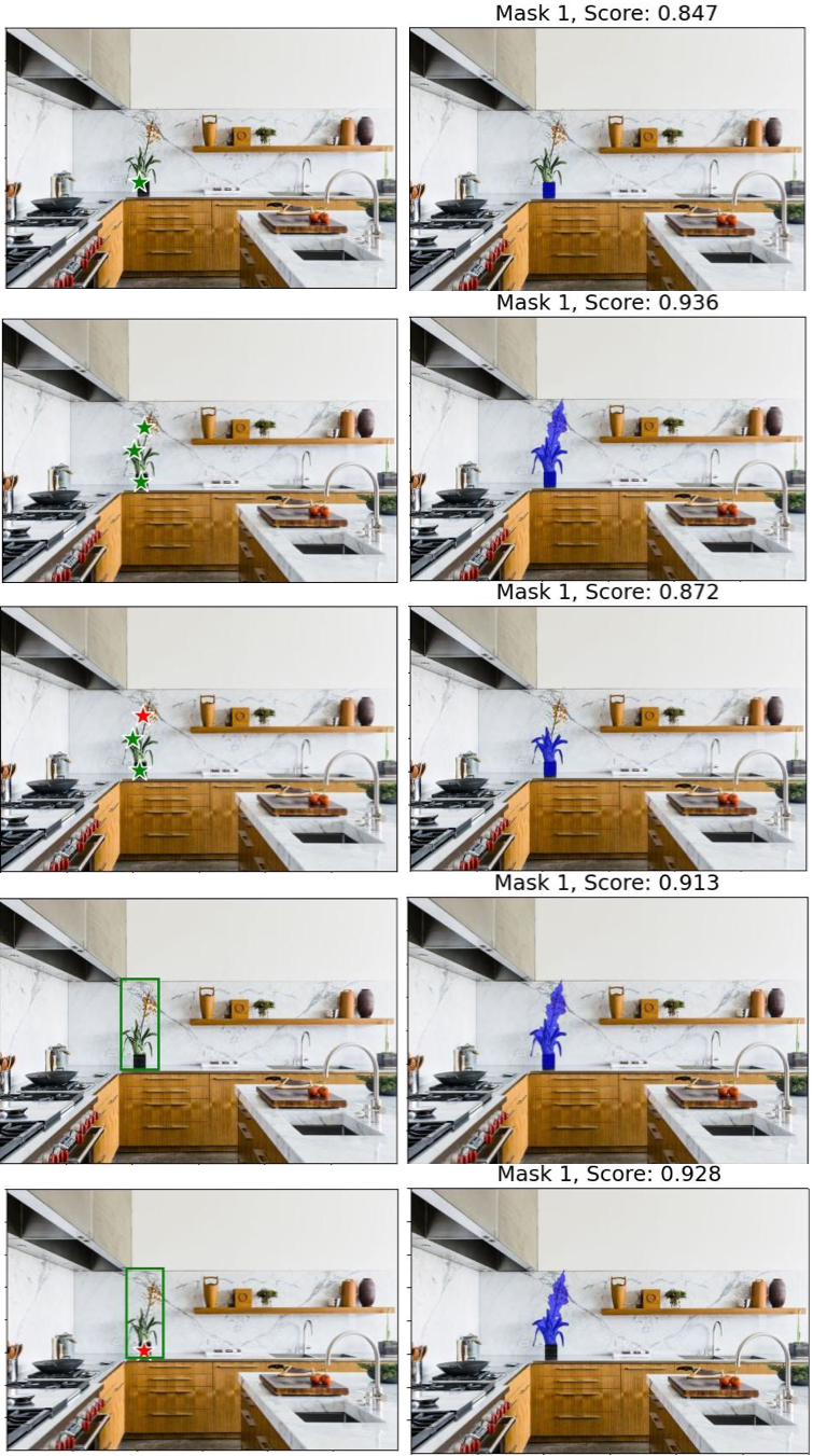
Let us discuss in detail the results shown in Figure 2.

In row 1, we notice that we have a single point as prompt (left), and we notice that SAM outputs a segmentation mask (right, in blue) which segments out the pot region on which the point lies.

In row 2, we notice that we have three points that span the plant with pot on the slab, and SAM correctly outputs a segmentation mask (right, in blue) which segments out the entire plant region on which the points lie.

In row 3, we notice that we have three points, out of which we want to segment a region such that the 2 points are included, and the third red point on the brown branch is excluded. Notice that SAM shows amazing results for this prompt as it correctly segments the whole plant region except the brown branch part where the red point lies.

In row 4, we simply provide a bounding box as a prompt and notice that SAM easily segments out the plant inside the box.

Finally, in row 5, we use a combination of bounding box and point coordinates where we want to segment the object within the bounding box but exclude the pot region where the red point lies. Note that the SAM prediction captures these intricate details of the prompts and segments out the plant except the pot region, as shown on the right.

Engineering different prompts allows us to control the SAM predictions to better segment the regions of interest.

---

Segmenting with SAM and Text Prompts

In the previous section, we discussed using point coordinates and bounding boxes to make predictions using the promptable SAM.

The original SAM paper (link) also mentioned that SAM can use text prompts to segment desired objects. However, the current release of the official code and models do not directly support segmentation with text prompts.

In this section, we will tackle this by using an off-the-shelf model and integrating it with our SAM pipeline.

The Grounding DINO model (link) takes in a text prompt and an image and outputs bounding box coordinates in the image corresponding to the object described by the text. For example, given that we provide a text prompt dog, the Grounding DINO model will simply output boxes bounding the regions where dogs occur in that image.

Note that this allows us to build a simple interface with SAM where we can provide a text prompt to the off-the-shelf Grounding DINO model, and it will output bounding boxes corresponding to that text which can then be directly used to prompt SAM, as we discussed in the previous section.

Let us go ahead and open the gdino_integration.py file to see this in action.

# USAGE: python gdino_integration.py

import cv2
import numpy as np
import torch
from groundingdino.util.inference import load_image, load_model, predict
from segment_anything import SamPredictor, sam_model_registry

from pyimagesearch import config
from sam import visualize_and_save_segmentation


def get_bounding_boxes(img_path, text_prompt, box_threshold, text_threshold):
    # Load GDINO model and input image
    model = load_model(config.GDINO_CONFIG, config.GDINO_CHECKPOINT_PATH)
    _, image = load_image(img_path)

    boxes, _, _ = predict(
        model=model,
        image=image,
        caption=text_prompt,
        box_threshold=box_threshold,
        text_threshold=text_threshold,
    )

    return boxes

We start by importing the OpenCV library (Line 3), the numpy library (Line 4), and the pytorch library (Line 5).

Next, we import SAM and the corresponding modules (as discussed above) and the Grounding DINO modules on Lines 6 and 7. Furthermore, we import the config file and the visualize_and_save_segmentation function defined above in the sam.py file on Lines 9 and 10.

Now that we have imported the necessary packages, we implement the get_bounding_boxes() function (Lines 13-26), using the Grounding DINO model to predict a bounding box based on the text prompt we provide.

The function takes as input the image path, the text prompt, and the threshold for the bounding box and text that the Grounding DINO model expects, as shown on Line 13.

We use the load_model function to initialize and load the Grounding DINO model. This function takes as input the path to the Grounding DINO config file and the path to the pre-trained checkpoint (i.e., config.GDINO_CONFIG, config.GDINO_CHECKPOINT_PATH), as shown on Line 15.

Next, use the load_image function, which takes as input the img_path and outputs the image in the format expected by the Grounding DINO model (Line 16).

Then, we call the predict function from Grounding DINO to get the bounding box corresponding to the object in the text prompt. The predict function takes as input the pre-trained model, the input image, the text_prompt corresponding to the object to detect, and the box_threshold and text_threshold scores to be used by the grounded DINO model for the predictions (Lines 18-24).

Finally, we return the set of bounding boxes (i.e., boxes) predicted by the grounded DINO model corresponding to the text prompt we provided (Line 26).

This completes the implementation of our get_bounding_box function, and we are now ready to make predictions with our models.

if __name__ == "__main__":
    # Load input image and convert to RGB
    print("[INFO] Loading image...")
    image = cv2.imread(config.IMG_PATH[0])
    image = cv2.cvtColor(image, cv2.COLOR_BGR2RGB)
    W, H = image.shape[1], image.shape[0]

    # Initialize and load SAM
    print("[INFO] Loading SAM model...")
    sam = sam_model_registry[config.MODEL_TYPE](checkpoint=config.SAM_CHECKPOINT_PATH)
    predictor = SamPredictor(sam)
    predictor.set_image(image)

    # Process text prompts
    print("[INFO] Generating masks from SAM...")
    for prompt_text in config.TEXT_PROMPT:
        # Get bounding boxes for the given prompt
        boxes = get_bounding_boxes(
            config.IMG_PATH[0], prompt_text, config.BOX_TRESHOLD, config.TEXT_TRESHOLD
        )

        for index, bbox in enumerate(boxes):
            # Preprocess bounding box
            box = torch.Tensor(bbox) * torch.Tensor([W, H, W, H])
            box[:2] -= box[2:] / 2
            box[2:] += box[:2]
            x0, y0, x1, y1 = box.int().tolist()

            # Prepare SAM prompt
            input_box = np.array([x0, y0, x1, y1])
            input_point = None
            input_label = None
            segment_prompt = [input_point, input_label, input_box]

            # Segment using the prepared prompt
            visualize_and_save_segmentation(segment_prompt, predictor, index)

We start by loading our image using OpenCV from the path defined by config.IMG_PATH[0] and converting it from the BGR to RGB color space using the cv2.cvtColor function, as shown on Lines 32 and 33. We also obtain our input image’s width and height dimensions, as shown on Lines 34.

Next, we initialize our SAM using sam_model_registry with the type of model (i.e., config.MODEL_TYPE) as discussed above. Furthermore, we also provide the path where we stored the SAM checkpoint (i.e., config.SAM_CHECKPOINT_PATH), as shown on Line 38.

On Lines 39 and 40, we get the predictor using the SamPredictor() module and use the predictor.set_image functionality to set our image as the input to SAM.

Now that we have the SAM and our input image set up, we can take the text prompts as input and make predictions using our integrated Grounding DINO and SAM pipeline in real-time.

We will test our pipeline by making predictions for each of the three text entries in our config.TEXT_PROMPT list (i.e., plant, apples, vase) one by one.

We start by iterating over the entries in config.TEXT_PROMPT (Line 44), and for each entry, we get the corresponding set of bounding boxes by calling the get_bounding_boxes() function, which we defined on Line 46.

Note that there might be multiple bounding boxes corresponding to the given object in the text prompt, as that object might have multiple instances in the image.

Then we iterate over each bbox in the boxes list (Line 47). For each bbox, we multiply the output coordinates with torch.Tensor([W, H, W, H]) (Line 52). Next, we process the coordinates as shown on Lines 53 and 54 to get the box coordinates.

Then we get the x, y coordinates from the box and convert them to integer values, as shown on Line 55.

Now that we have the bounding box coordinates for the object in the given text prompt, we create a numpy array and store them as input_box, as shown on Line 58. Furthermore, we set the input_point and input_label to None (Lines 59 and 60) and create our prompt list, which the visualize_and_save_segmentation function takes, as discussed in detail above.

Finally, we use the visualize_and_save_segmentation() function, which takes as input the SAM predictor and the prompt along with the index to output segmentation masks.

Figure 3 shows the results of our text prompt segmentation pipeline.

In row 1, we notice that Grounding DINO predicted the bounding box for the plant text prompt, that is, the small plant on the top shelf, and SAM segmented the plant (right) perfectly.

Similarly, in row 2, Grounding DINO predicted the bounding box for the apple text prompt, that is, the small apple near the tap, and SAM segmented the apple (right, blue color) very well. Notice that this is a pretty amazing result since the apple is very small and not clearly visible in the image.

Finally, in row 3, Grounding DINO predicted the bounding box for the vase text prompt, that is, the vase below the potted plant, and SAM segmented exactly the vase (right, blue color) part, excluding the plant.

After visualizing these results, we can clearly see that SAM has amazing capabilities as a foundational segmentation model and can be used to segment various objects in any image in a zero-shot way without fine-tuning.

---

---

Summary

In this tutorial, we tried to gain a holistic understanding of SAM, a foundational segmentation model. Specifically, we discussed SAM’s development and pre-training process and implemented code to predict segmentation masks using different prompts.

Furthermore, we discussed how different prompts can be combined to prompt SAM and get control over the desired region to segment in input images.

Finally, we discussed how SAM can seamlessly be integrated with the off-the-shelf Grounding DINO model to segment objects with text-based prompts.

In the next tutorial, we will further understand how SAM can be integrated with other systems and used to perform diverse downstream tasks.

---

Credits

This blog post is inspired by the official SAM paper and GitHub code release for SAM (https://github.com/facebookresearch/segment-anything) and Grounding DINO (https://github.com/IDEA-Research/GroundingDINO).

---

Citation Information

Chandhok, S. “SAM from Meta AI (Part 1): Segmentation with Prompts,” PyImageSearch, P. Chugh, A. R. Gosthipaty, S. Huot, K. Kidriavsteva, and R. Raha, eds., 2023, https://pyimg.co/0ivy4

@incollection{Chandhok_2023_SAM-Part1,
  author = {Shivam Chandhok},
  title = {{SAM} from {Meta AI} (Part 1): Segmentation with Prompts},
  booktitle = {PyImageSearch},
  editor = {Puneet Chugh and Aritra Roy Gosthipaty and Susan Huot and Kseniia Kidriavsteva and Ritwik Raha},
  year = {2023},
  url = {https://pyimg.co/0ivy4},
}

---

---

To download the source code to this post (and be notified when future tutorials are published here on PyImageSearch), simply enter your email address in the form below!

The post SAM from Meta AI (Part 1): Segmentation with Prompts appeared first on PyImageSearch.

Find A Teacher Form:
https://docs.google.com/forms/d/1vREBnX5n262umf4wU5U2pyTwvk9O-JrAgblA-wH9GFQ/viewform?edit_requested=true#responses

Email:
public1989two@gmail.com






www.itsec.hk
www.itsec.vip
www.itseceu.uk