SAM from Meta AI (Part 2): Integration with CLIP for Downstream Tasks

---

Table of Contents

---

SAM from Meta AI (Part 2): Integration with CLIP for Downstream Tasks

In this tutorial, you will learn about the Segment Anything Model (SAM) from Meta AI and understand how it can be integrated with other foundational models like CLIP (contrastive language-image pretraining) to tackle a diverse range of downstream tasks like zero-shot image classification, text-to-image retrieval and image similarity.

This lesson is the last of a 2-part series on Segment Anything Model (SAM) from Meta AI:

1. SAM from Meta AI (Part 1): Segmentation with Prompts
2. SAM from Meta AI (Part 2): Integration with CLIP for Downstream Tasks (this tutorial)

To learn how to integrate SAM with CLIP for downstream tasks, just keep reading.

---

SAM from Meta AI (Part 2): Integration with CLIP for Downstream Tasks

In the first part of this series, we discussed the development of “foundational models,” which are trained on large-scale datasets and possess more “general” capabilities that allow them to understand data holistically and perform various downstream tasks of varied data distributions.

We took an in-depth look at the SAM, which is a foundational segmentation model, and tried to develop a holistic understanding of SAM.

The two most important characteristics of SAM that we discussed were its ability to perform segmentation on data from a variety of distributions with prompt engineering and that it can be seamlessly integrated with pre-established computer vision models and systems to boost their capabilities and performance on complex tasks for which training task-specific models would not be feasible.

In the previous tutorial, we discussed the former in detail to understand how SAM can be prompted in different ways to segment specific regions in any image in real-time. In this tutorial, we will focus on the latter and discuss how SAM can be integrated with other foundational models like CLIP to perform a range of downstream tasks (e.g., zero-shot image classification, text-to-image retrieval, and image similarity).

---

SAM and CLIP Integration

As we briefly discussed in the previous tutorial, the CLIP model is a recent foundational model for computer vision that utilizes large-scale web-based image-text data to train strong representations that encode semantic knowledge. The image and text instances are directly scraped from the web and are weakly aligned (e.g., image and tags on the web), which allows us to train this model with low annotation cost.

The CLIP model consists of an image encoder and a text encoder. The image encoder takes an image as input and maps it to an N-dimensional representation space. Similarly, the text encoder takes as input the corresponding text and maps it to the same N-dimensional representation space. Then, a contrastive objective is used to align corresponding image and text pairs and push dissimilar image and text pairs apart to learn useful semantic representations.

Let us now take an example and understand how our SAM+CLIP system can help us perform complex and diverse downstream tasks.

Suppose we have an image I with multiple objects, and we want to classify each object in the image into a set of categories in a zero-shot way (i.e., without using any data to train the model).

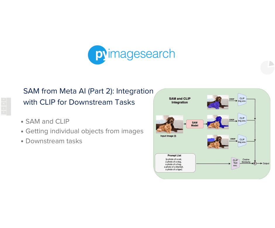
Figure 1 shows an overview of a pipeline that integrates SAM with the CLIP model to perform this task seamlessly.

The input image I is passed through SAM, which is used in a mode that extracts and outputs all plausible segmentation masks for objects in that image. Then, these individual objects are cropped out of the image and preprocessed to pass them through the pre-trained CLIP image encoder, which maps them to an N-dimensional representation.

Similarly, the text prompts are passed as input to the pre-trained CLIP text encoder, which maps them to an N-dimensional representation. Since CLIP is trained in a way that the output of the text and image encoder are aligned in the N-dimensional space, we can use cosine similarity between the cropped object representation and the prompt representation and classify the objects in the image by matching it with the most similar prompt from the prompt list as shown.

Similarly, this integration system can be used for various other tasks (e.g., text-to-image retrieval, image similarity, etc.), as detailed in this tutorial.

---

Configuring Your Development Environment

To follow this guide, you need to have the SAM and CLIP model. Furthermore, you will need to download the pre-trained checkpoints for these models.

Luckily, this can be done easily by following the commands below:

$ pip install
git+https://github.com/facebookresearch/segment-anything.git
$ pip install opencv-python pycocotools matplotlib onnxruntime onnx
$pip install open_clip_torch

$ mkdir checkpoints
$ cd checkpoints
$ wget -c https://dl.fbaipublicfiles.com/segment_anything/sam_vit_h_4b8939.pth

If you need help configuring your development environment for OpenCV, we highly recommend that you read our pip install OpenCV guide — it will have you up and running in minutes.

---

Need Help Configuring Your Development Environment?

All that said, are you:

• Short on time?
• Learning on your employer’s administratively locked system?
• Wanting to skip the hassle of fighting with the command line, package managers, and virtual environments?
• Ready to run the code immediately on your Windows, macOS, or Linux system?

Then join PyImageSearch University today!

Gain access to Jupyter Notebooks for this tutorial and other PyImageSearch guides pre-configured to run on Google Colab’s ecosystem right in your web browser! No installation required.

And best of all, these Jupyter Notebooks will run on Windows, macOS, and Linux!

---

Project Structure

We first need to review our project directory structure.

Start by accessing this tutorial’s “Downloads” section to retrieve the source code and example images.

From there, take a look at the directory structure:

├── checkpoints
├── clip_integration.py
├── config.py
├── gdino_integration.py
├── get_objects.py
├── images
│   ├── kitchen.jpeg
│   └── living_room.jpg
├── sam.py
└── utils.py

In the previous tutorial, we discussed in detail the directory structure and the function of each file.

Specifically, we discussed the checkpoints and images folder, which stores the pre-trained checkpoints and images we will use for the tutorial. Furthermore, we discussed the config.py, gdino_integration.py, sam.py, and utils.py files in detail.

In this tutorial, we will take an in-depth look at the get_objects.py file, which implements the code to extract segmentation masks for objects in the input image and then crop them for our downstream tasks.

Additionally, we will walk through the clip_integration.py file, which implements the code for our SAM and CLIP integrated system and performs tasks (e.g., zero-shot object classification, text-to-image retrieval, and image similarity).

---

Getting Individual Objects from Image

In this section, we discuss how we can extract different objects in our input image so we can use them later for performing our downstream recognition and retrieval tasks.

In the previous tutorial, we discussed how SAM can be prompted to segment regions or objects of interest. This can be referred to as the promptable segmentation mode for SAM.

Another more general mode in which SAM can be used is to generate all plausible segmentation masks in a given input image. This can be done with the SamAutomaticMaskGenerator functionality, where SAM takes an input image, predicts plausible segmentation masks, and estimates bounding boxes corresponding to each mask.

Let us go ahead and discuss how this can be implemented in code and how we can use this functionality of SAM to segment and crop out prominent objects in our input image.

We open the get_objects.py file and get started.

# USAGE: python get_objects.py

# Import the necessary packages
import os
import pickle

import cv2
import matplotlib.pyplot as plt
from segment_anything import SamAutomaticMaskGenerator, sam_model_registry

from pyimagesearch import config, utils


def generate_object_masks(image):
    # Initialize SAM model and generate masks
    print("[INFO] Loading SAM model...")
    sam = sam_model_registry[config.MODEL_TYPE](checkpoint=config.SAM_CHECKPOINT_PATH)
    mask_generator = SamAutomaticMaskGenerator(sam)
    masks = mask_generator.generate(image)

    return masks


def save_object_crops(masks, mask_ids, labels):
    # Crop objects from image using mask IDs and save
    obj_crops = []
    for id in mask_ids:
        box = masks[id]["bbox"]
        x0, y0, w, h = box
        crop = image[y0 : y0 + h, x0 : x0 + w]
        obj_crops.append(crop)

    # Save object crops and corresponding labels
    obj_dict = {"crops": obj_crops, "labels": labels}
    with open(os.path.join(config.OUT_PATH, "objects.pkl"), "wb") as fp:
        pickle.dump(obj_dict, fp)

We start by importing the os module, and the pickle package (Lines 4 and 5). Next we import the OpenCV and Matplotlib libraries, as shown on Lines 7 and 8, respectively. On Line 9, we import necessary modules that will allow us to use SAM for making predictions in our tutorial. Specifically, we get the SamAutomaticMaskGenerator and sam_model_registry modules from segment_anything, as shown on Line 9.

Finally we import the config file, which stores the initial configurations of our parameters (Line 11) and the utils.py file, which implements the helper functions to visualize the segmentation masks from SAM (Line 11).

Now that we have imported the necessary modules and packages, it is time to implement our get_object_masks function (Lines 14-21), which takes the input image and uses the pre-trained SAM to predict and automatically generate masks for the entire image.

We first initialize SAM using the sam_model_registry functionality with the type of model (i.e., config.MODEL_TYPE), which we take as vit_h for this tutorial. Further, we provide the path where we stored the SAM checkpoint (i.e., config.SAM_CHECKPOINT_PATH), as shown on Line 17.

On Line 18, we get the mask_generator using the SamAutomaticMaskGenerator module, allowing us to automatically extract masks for the different objects in our input image.

Finally, on Line 19, we use the generator functionality of the mask_generator object that we created to get the masks for the entire image and return the predicted masks on Line 21.

Now that we have completed the definition of our get_object_masks function, discuss the save_object_crops function which will allow us to crop out everyday objects detected by SAM from our input image and save them with their corresponding labels. This will further help us perform the downstream tasks we want with the different objects in our image as we will see later.

We first initialize an empty obj_crops list (Line 26), where we will store our object crops. Then, for each ID in our mask_ids list, we get the bounding box predicted by SAM (Line 28) and get the corresponding x0, y0 coordinates and width and height (Line 29).

Next, we use the coordinates to get the part or crop of the image with the particular object (Line 30) and add it to our obj_crops list (Line 31).

Finally, we create a dictionary named obj_dict and store the obj_crops list and the corresponding labels, as shown on Line 34. Then, we save this dictionary with the filename objects.pkl in the config.OUT_PATH folder (Line 35).

if __name__ == "__main__":
    # Load input image and convert to RGB
    print("[INFO] Loading image...")
    image = cv2.imread(config.IMG_PATH[1])
    image = cv2.cvtColor(image, cv2.COLOR_BGR2RGB)

    # Generate segmentation masks
    print("[INFO] Generating masks from SAM...")
    all_masks = generate_object_masks(image)

    # Create output directory if it doesn't exist
    if not os.path.exists(config.OUT_PATH):
        os.makedirs(config.OUT_PATH)

    # Plot and save predicted image
    prediction_path = os.path.join(config.OUT_PATH, config.OUT_PRED_PATH)
    plt.figure(figsize=(8, 8))
    plt.imshow(image)
    utils.show_all_masks(all_masks)
    plt.savefig(prediction_path)

    # Plot individual object masks
    for i, mask_info in enumerate(all_masks):
        plt.figure(figsize=(6, 6))
        plt.imshow(image)
        utils.show_mask(mask_info["segmentation"], plt.gca())
        plt.axis("off")
        plt.savefig(os.path.join(config.OUT_PATH, f"mask_{i}.png"))

    # TODO: Place mask and labels in the config
    mask_ids = [0, 2, 3, 7, 8, 11, 12, 20, 22, 23, 26, 27, 34, 35, 45, 66, 67, 78]
    labels = [
        "painting",
        "door",
        "painting",
        "carpet",
        "vase",
        "plant",
        "pillow",
        "blanket",
        "pillow",
        "pillow",
        "blanket",
        "jug",
        "blanket",
        "dog",
        "plant",
        "plant",
        "plant",
        "pillow",
    ]

    # Save object crops and corresponding labels
    print("[INFO] Cropping and saving objects...")
    save_object_crops(all_masks, mask_ids, labels)

Next, let us go ahead and implement the main function to see our model in action.

We start by loading our image using OpenCV from the path defined by config.IMG_PATH[1] and converting it from BGR to RGB color space using the cv2.cvtColor function, as shown on Lines 42 and 43.

Next, on Line 47, we use the get_object_masks function that we defined above to extract the segmentation masks from our input image and store it as all_masks. Notice that the all_masks output from SAM is a dictionary with the following keys: [‘segmentation’, ‘area’, ‘bbox’, ‘predicted_iou’, ‘point_coords’, ‘stability_score’, ‘crop_box’].

Note that we will use the segmentation masks (i.e., ‘segmentation’ key) and the bounding box (i.e., ‘bbox’ key) for cropping individual objects.

Now that we have the SAM predictions, let us prepare to visualize them on our input image and save the final visualizations.

We first check if the folder where the output predictions will be stored (i.e., config.OUT_PATH) already exists, and if not, we create it (Lines 50 and 51). Furthermore, we define the prediction_path on Line 54, which indicates the location where our segmentation visualization will be stored.

On Lines 55 and 56, we initialize a matplotlib figure and visualize the input image.

Next, we visualize all the predicted segmentation masks from SAM using the show_all_masks function and save the visualization using the plt.savefig at the prediction_path, as shown on Lines 57 and 58.

Figure 2 shows the visualization of all segmentation masks predicted by SAM for our input image.

Now, let us go ahead and visualize each segmentation mask and the corresponding bounding box predicted by SAM to get a sense of the prominent objects that were segmented out by SAM.

We start by iterating over the all_masks output. For each segmentation prediction, we first plot the input image (Lines 62 and 63) and then visualize the segmentation mask (i.e., mask_info['segmentation']) using the show_mask function (Lines 64 and 65).

Finally, we save the visualization using the plt.savefig in the config.OUT_PATH folder, as shown on Line 66.

Now that we have visualized each prediction and their corresponding segmentation masks and bounding boxes, let us take a list of predicted mask IDs from SAM with prominent everyday objects and the corresponding object names or labels (Line 69).

Note that on Line 69-89, we manually curate a few mask IDs (which we visualized) with prominent everyday objects (e.g., paintings, plants, vases, pillows, etc.) and assign them corresponding labels with the help of the labels list.

Finally we use the save_object_crops function that we defined above to save the object crops.

We will use these objects extracted from our input image for our downstream tasks.

Figure 3 shows a few examples of cropped objects and their corresponding labels.

---

Downstream Tasks with SAM and CLIP

Now that we have extracted individual objects from our input image, it is time to complete building our SAM and the CLIP-based system and use it for the aforementioned downstream tasks.

Specifically, we will take the cropped objects stored in the previous section and pass them through the pre-trained CLIP image encoder model. Additionally, we will engineer prompts for our labels and pass them through the pre-trained CLIP text encoder model to get N-dimensional (here 512-dimensional) representations.

Then, we will use cosine similarity to classify images or retrieve them based on text prompts, as discussed below.

Let us open our clip_integration.py file and get started.

# USAGE
# python clip_integration.py

# import the necessary packages
from pyimagesearch import config
import matplotlib.pyplot as plt
import open_clip
import pickle
import torch
import PIL
import os

def compute_clip_features(model, tokenizer, image, prompts):
    """Compute CLIP features for given image and prompts"""

    # tokenize the text
    text = tokenizer(prompts)

    # compute CLIP image and text features
    with torch.no_grad(), torch.cuda.amp.autocast():
        image_features = model.encode_image(image)
        text_features = model.encode_text(text)
        image_features /= image_features.norm(dim=-1, keepdim=True)
        text_features /= text_features.norm(dim=-1, keepdim=True)

    # return image and text features
    return (image_features, text_features)

if __name__ == "__main__":
    # load object crops and labels
    print("[INFO] Loading object crops...")
    with open(os.path.join(config.OUT_PATH, "objects.pkl"), "rb") as fp:
        obj_dict = pickle.load(fp)
        obj_crops = obj_dict["crops"]
        labels = obj_dict["labels"]

    # get unique objects
    print("[INFO] Getting unique objects...")
    objects = set(labels)

    # initialize CLIP model
    print("[INFO] Loading CLIP model...")
    model, _, preprocess = open_clip.create_model_and_transforms(
        "ViT-B-32", pretrained="laion2b_s34b_b79k"
    )
    tokenizer = open_clip.get_tokenizer("ViT-B-32")

    # create prompts
    print("[INFO] Creating prompts...")
    prompts = ["a photo of a " + item for item in objects]

We start by importing the necessary packages as always on Lines 5-11.

Next, we define the compute_clip_features function, which takes as input the pre-trained CLIP model, the corresponding text tokenizer, the input image, and the list of prompts and outputs the image features and text features or representations from CLIP (Lines 13-27).

On Line 17, we start by using the tokenizer to convert the text prompts into corresponding tokens, which can be input to the text encoder of CLIP. Next, we switch off the gradient computation (Line 20) (as we are using a pre-trained CLIP model for inference only) and encode the image and the text by passing it through the CLIP model using the encode_image and encode_text functions (Lines 21 and 22).

Finally, we normalize image_features and text_features to have unit norm and return them on Lines 23 and 24.

Now that we have implemented the function to get the CLIP features, let us load the cropped objects we saved in the previous section and prepare for implementing the downstream tasks.

We start by opening the objects.pkl file from the config.OUT_PATH folder (Line 32) and loading the saved obj_dict dictionary (Line 33). Next, we get the obj_crops and labels list we created in the previous section (Lines 34 and 35). We use the set() functionality to get a list of unique objects from our labels list (Line 39).

It is now time to initialize and load our pre-trained CLIP model. Note that for this tutorial, we will use the Open CLIP implementation and weights.

On Lines 43 and 44, we initialize the open_clip ViT-B-32 architecture-based model and load the laion2b_s34b_b79k pre-trained weights. This allows us to get the model and preprocess transformations (Line 43), which we will apply to our input image before passing it through the image encoder of the CLIP model. Furthermore, on Line 46, we get the text tokenizer for ‘ViT-B-32’, which will allow us to preprocess the text and convert it to tokens, which can be fed to the text encoder of CLIP.

Then, we engineer prompts for each object in our unique objects list. The simplest way to engineer prompts for CLIP is to simply have a sentence like ‘a photo of a {}’ and replace the {} with the object name.

On Line 50, we create a prompt for each object with the above format.

# initialize list to store all processed images
    images_all = []

# loop over all objects and perform zero-shot image classification
for (i, crop) in enumerate(obj_crops):
        # pre-process the image and compute both image and text
        # features
        image = PIL.Image.fromarray(crop)
        image_processed = preprocess(image).unsqueeze(0)
        images_all.append(image_processed)
        image_features, text_features = compute_clip_features(model,
            tokenizer, image_processed, prompts)

        # calculate the similarity and display it
        similarity = image_features @ text_features.T
        probs = (100.0 * similarity).softmax(dim=-1)
        print("Object is", prompts[torch.argmax(probs).item()])

    # text to image retrieval
    images_all_tensor = torch.cat(images_all, axis=0)

    # loop over all prompts
    for (i, prompt) in enumerate(prompts):
        # compute features and calculate the similarity
        (image_features, text_features) = compute_clip_features(model,
            tokenizer, images_all_tensor, [prompt])
        similarity = image_features @ text_features.T
        probs = (100.0 * similarity).softmax(dim=-1)
        max_crop = obj_crops[torch.argmax(probs).item()]

        # plot the image and save to disk
        plt.figure(figsize=(1, 1))
        plt.imshow(max_crop)
        plt.savefig(os.path.join(config.OUT_PATH, "obj_" + str(i) + ".png"))

    # calculate and display image similarity
    img_embed, _ = compute_clip_features(model, tokenizer,
        images_all_tensor, [prompts[0]])
    sim = img_embed @ img_embed.T
    print(sim)

Now that we have our prompts and pre-trained CLIP model ready, it is time to go ahead and see our pipeline perform different downstream tasks.

Let us start with zero-shot classification of the objects we extracted from the image using SAM.

In this task, we take one object crop at a time and use CLIP to identify which prompt sentence from the prompts list best describes the object.

We start by initializing an empty images_all list which will store all processed images later.

For each cropped object image in the obj_crops list, we first convert the numpy array to a PIL image (Line 59) and use the preprocess function from Open CLIP to get the image in the format expected by the image encoder of CLIP (Line 60). We store this processed image in the images_all list, as shown on Line 61.

Next, we pass the CLIP model, tokenizer, processed image (i.e., image_processed) and prompts list as arguments to the get_clip_features function we defined above and get the corresponding image_features and text_features (Lines 62 and 63).

Notice that image_features is the CLIP image encoder representation for the current cropped object under consideration (with dimension [1, 512]) and text_features is the CLIP text encoder representation for all 9 prompts in the prompts list (with dimension [9, 512]).

Since the image_features and text_features are in the same latent space, we can simply compute the cosine similarity of image_features with text_features of each prompt.

Since both image_features and text_features have unit norms, the cosine similarity can be easily calculated by simply taking the outer product of matrices (i.e., image_features @ text_features.T), as shown on Line 66.

Furthermore, to convert the similarity scores to probabilities, we scale them by multiplying them by 100 and taking softmax, as shown on Line 67.

This gives us 9 probability values, each indicating the similarity of the prompt sentence representation with the image representation.

On Line 68, we take the prompt with the maximum probability as the description or class of the object in the image crop.

Next, let us move on to the text-to-image retrieval task. For this task, our job is to take one prompt in our prompts list at a time and get the particular object crop (from all object crops we have), which matches the prompt.

First, we consolidate all our object crops and preprocess them to a format that the CLIP image encoder expects and put them together in a list.

On Line 71, we consolidate by concatenating all the elements in the images_all list.

We are now ready to perform our text-to-image retrieval task.

For each prompt in our prompt list, we iterate through one by one (Line 74) and pass the CLIP model, tokenizer, images_all tensor, and the specific prompt (i.e., [prompts[i]]) to the compute_clip_features function (Lines 76 and 77), which outputs the image_features and text_features.

Notice that the image_features here is the CLIP image encoder representation for all cropped objects (with dimension [18, 512]), and text_features is the CLIP text encoder representation of the particular prompt under consideration (with dimension [1, 512]).

Once we have the representations, we follow the procedure we did in our zero-shot classification experiment.

As both image_features and text_features have unit norms, the cosine similarity can be easily calculated by simply taking the outer product of matrices (i.e., image_features @ text_features.T) as shown on Line 78.

Furthermore, to convert the similarity scores to probabilities, we scale them by multiplying with 100 and take softmax, as shown on Line 79.

This gives us 18 probability values, each indicating the similarity of the given prompt sentence with the 18 object crops.

On Line 80, we take the crop from the obj_crops list with the maximum probability assigned (i.e., max_crop) for the given prompt and plot it using matplotlib on Lines 83 and 84. Finally, on Line 85, we save this object crop.

Let us now move to our image similarity task, where our job will be to find out which object crops in our list obj_crops are the most similar.

Note that in both the previous tasks, we used both the CLIP image and text encoders to get scores since these tasks were based on both the image and text modality.

However, we only need the CLIP image encoder for the image similarity task, as this task only involves visual modality and not text modality.

On Line 88, we simply use the compute_clip_features function, which takes our model, tokenizer, tensor with all our images, and a dummy prompt. Note that we can pass any prompt here since we are only interested in using the image encoder to get image features, and we will not use the text or text encoder features at all for this task.

We store the image embeddings or features as img_embed, as shown on Line 88.

Next, we want to compute the similarity score between each pair of object crops or images.

This can simply be done using the outer product between img_embed and img_embed transpose, as shown on Line 90.

Let us consider a few examples of crops we saw above and try to understand the sim similarity matrix for these crops that our code generates.

Figure 4 shows the image similarities for a few crops we considered in the previous section.

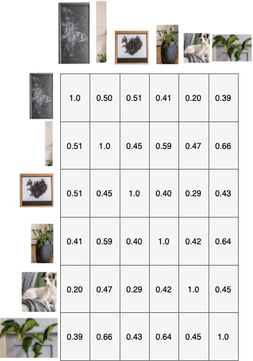
Notice that semantically similar objects have high similarity scores. Also, note that the similarity of an image crop with itself (on the diagonal) is always 1.0.

In row 1, we notice that the painting crop is most similar to (apart from itself) the crop of another painting. In row 3, we also notice the same thing with the other painting.

In row 4, we notice that the plant crop is most similar to (apart from itself) the crop of another plant as shown. We also notice the same thing in row 6.

This completes our implementation for performing various downstream tasks with SAM and the CLIP-based system we discussed at the beginning of the tutorial.

---

---

Summary

In this tutorial, we looked at how SAM can be integrated with existing models to build systems that can perform diverse downstream tasks without fine-tuning the models using a task-specific curated dataset.

Specifically, we built our own SAM and CLIP-based pipeline in PyTorch, which can extract objects of interest from images and perform classification or text-to-image retrieval in a zero-shot fashion on the extracted individual objects.

The two tutorials in this series show the amazing capabilities of SAM and discuss the various ways that SAM can be used in your own computer vision for solving segmentation or other diverse downstream tasks.

---

Citation Information

Chandhok, S. “SAM from Meta AI (Part 2): Integration with CLIP for Downstream Tasks,” PyImageSearch, P. Chugh, A. R. Gosthipaty, S. Huot, K. Kidriavsteva, and R. Raha, eds., 2023, https://pyimg.co/27uny

@incollection{Chandhok_2023_SAM-Part2,
  author = {Shivam Chandhok},
  title = {{SAM} from {Meta AI} (Part 2): Integration with {CLIP} for Downstream Tasks},
  booktitle = {PyImageSearch},
  editor = {Puneet Chugh and Aritra Roy Gosthipaty and Susan Huot and Kseniia Kidriavsteva and Ritwik Raha},
  year = {2023},
  url = {https://pyimg.co/27uny},
}

---

---

To download the source code to this post (and be notified when future tutorials are published here on PyImageSearch), simply enter your email address in the form below!

The post SAM from Meta AI (Part 2): Integration with CLIP for Downstream Tasks appeared first on PyImageSearch.

Find A Teacher Form:
https://docs.google.com/forms/d/1vREBnX5n262umf4wU5U2pyTwvk9O-JrAgblA-wH9GFQ/viewform?edit_requested=true#responses

Email:
public1989two@gmail.com






www.itsec.hk
www.itsec.vip
www.itseceu.uk