A Deep Dive into Variational Autoencoders with PyTorch

---

Table of Contents

---

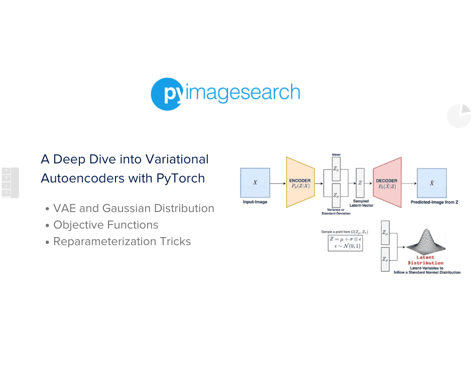
A Deep Dive into Variational Autoencoder with PyTorch

In this tutorial, we dive deep into the fascinating world of Variational Autoencoders (VAEs). We’ll start by unraveling the foundational concepts, exploring the roles of the encoder and decoder, and drawing comparisons between the traditional Convolutional Autoencoder (CAE) and the VAE. A special emphasis will be placed on the Gaussian distribution’s pivotal role in VAEs and the balance between reconstruction loss and KL divergence.

Using the renowned Fashion-MNIST dataset, we’ll guide you through understanding its nuances. As the tutorial progresses, you’ll delve into setting up prerequisites, crafting utilities, and designing the VAE network. The highlight will be the VAE training on the Fashion-MNIST data, followed by a detailed post-training analysis. This will encompass experiments ranging from latent space visualization to image generation. By the conclusion, you’ll have a deep appreciation for VAEs, their capabilities in image generation, and the intricacies of the dataset.

So, are you ready to delve into the captivating realm of VAEs with PyTorch? Let’s get started!

This lesson is the 3rd in a 5-part series on Autoencoders:

1. Introduction to Autoencoders
2. Implementing a Convolutional Autoencoder with PyTorch
3. A Deep Dive into Variational Autoencoders with PyTorch (this tutorial)
4. Lesson 4
5. Lesson 5

To learn the theoretical concepts behind Variational Autoencoder and delve into the intricacies of training one using the Fashion-MNIST dataset in PyTorch with numerous exciting experiments, just keep reading.

---

A Deep Dive into Variational Autoencoder with PyTorch

---

Introduction

Deep learning has achieved remarkable success in supervised tasks, especially in image recognition. However, in the realm of unsupervised learning, generative models like Generative Adversarial Networks (GANs) have gained prominence for their ability to produce synthetic yet realistic images. Before the rise of GANs, there were other foundational neural network architectures for generative modeling. One such model that predates the GAN era is the Variational Autoencoder (VAE).

In our previous tutorial on autoencoders, we learned that they are not inherently generative. While they can reconstruct input data effectively, they falter when generating new samples from the latent space unless specific points are manually chosen. This limitation was evident in experiments conducted on datasets like Fashion-MNIST.

VAEs were introduced in 2013 by Diederik et al. in their paper Auto-Encoding Variational Bayes. They extended the idea of autoencoders to learn useful data distributions. Rooted in Bayesian inference, VAEs aim to model the underlying probability distribution of data, enabling the generation of new samples from that distribution.

The key distinction between VAEs and traditional autoencoders is the design of their latent spaces. VAEs ensure continuous latent spaces, facilitating random sampling and interpolation, making them invaluable for generative modeling.

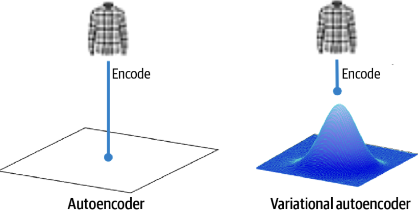
In a standard autoencoder, every image corresponds to a singular point within the latent space. Conversely, as shown in Figure 1, in a variational autoencoder, each image is associated with a multivariate normal distribution centered around a specific point in the latent space.

VAEs are a type of autoencoder, designed to learn efficient input data codings or representations. However, unlike traditional autoencoders that learn deterministic encodings, VAEs introduce a probabilistic twist. The encoder in a VAE doesn’t produce a fixed point in the latent space. Instead, it outputs parameters (typically mean and variance) of a probability distribution, which we sample to obtain our latent representation.

---

Comparison with Convolutional Autoencoder

---

Architecture

• Convolutional Autoencoder (CAE): A CAE typically consists of an encoder and a decoder. The encoder uses convolutional layers to compress the input into a compact latent representation, and the decoder uses transposed convolutional layers to reconstruct the input from this representation.
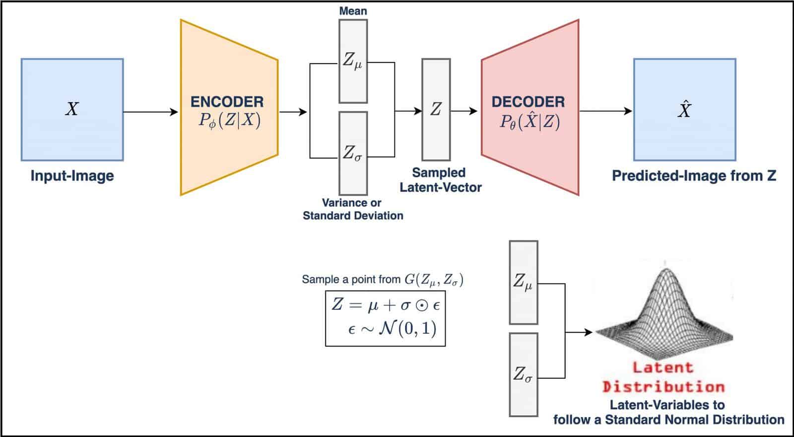
• VAE: Similar to a CAE, a VAE also has an encoder and a decoder. However, the encoder in a VAE produces parameters of a probability distribution (typically Gaussian) in the latent space rather than a deterministic point, as shown in Figure 2.

---

Latent Space

• CAE: The latent space in a CAE is deterministic. Given the same input, the encoder will always produce the same point in the latent space.
• VAE: The latent space in a VAE is probabilistic. The encoder produces a distribution’s parameters (mean and variance), and the actual latent representation is sampled from this distribution.

---

Loss Function

• CAE: The loss function of a CAE typically focuses on the reconstruction error, which measures the difference between the original input and its reconstruction.
• VAE: The VAE loss function has two components:
  • Reconstruction Loss: Like the CAE, this measures the fidelity of the reconstructed input.
  • Kullback-Leibler (KL) Divergence: This term ensures that the learned distribution in the latent space is close to a prior distribution, usually a standard Gaussian. It acts as a regularizer, preventing the model from encoding too much information in the latent space and ensuring smoothness in the latent space.

---

Why Does VAE Stand Out?

VAEs have garnered attention due to their ability to learn smooth and continuous latent spaces. This continuity ensures that small changes in the latent space result in coherent changes in the generated data, making VAEs suitable for tasks like interpolation between data points. Additionally, the probabilistic nature of VAEs introduces a level of randomness that can benefit generative tasks, allowing the model to produce diverse outputs.

---

Why Does the Encoder of a VAE Follow a Gaussian Distribution?

• Regularization and Continuity: The Gaussian distribution acts as a regularizer, ensuring the latent space is continuous. This continuity allows for smooth interpolations between data points, making it possible to generate new, similar data points by sampling from regions between known data points.
• Simplicity and Universality: The Gaussian distribution is mathematically tractable and is a universal approximator. VAEs can leverage their properties for efficient training and representation by constraining the latent variables to follow this distribution.
• Reparameterization Trick: The Gaussian distribution facilitates the reparameterization trick, a crucial component in VAEs. This trick allows for the backpropagation of gradients through the stochastic sampling process, enabling end-to-end training of the model.
• Balanced Latent Space: By pushing the encoder’s outputs to approximate a standard Gaussian distribution, VAEs prevent the model from assigning too much importance to any particular region of the latent space. This ensures a balanced representation where different regions of the space can be effectively utilized for data generation.

---

Objective Functions of VAE

VAEs optimize two primary loss functions:

Reconstruction Loss: This loss ensures that the images generated by the decoder closely resemble the input images. It’s typically computed using the Mean Squared Error (MSE) between the original and reconstructed images.

• represents the reconstruction loss.
• and are the parameters of the decoder and encoder, respectively.
• is the number of samples.
• is the original input image.
• is the decoder function, and is the encoder function.
• The formula calculates the squared difference between each original image and its corresponding reconstructed image , then averages these squared differences over all samples.

KL Divergence: This measures the difference between the encoder’s distribution and a standard normal distribution. It is a regularizer, ensuring the latent variables are close to a standard normal distribution. It encourages the model to maintain a structured and continuous latent space, which is particularly beneficial for generative tasks.

• represents the KL divergence loss.
• is the Gaussian distribution defined by the encoder’s outputs (mean) and (standard deviation).
• is the standard normal distribution.
• The formula calculates the difference between the encoder’s distribution and the standard normal distribution for each sample and sums these differences.

The combined VAE loss is a weighted sum of the reconstruction and KL divergence losses:

---

Reparameterization Trick

In the realm of Variational Autoencoder, one of the pivotal challenges is the integration of randomness in the latent space. This stochasticity, while essential for the VAE’s generative capabilities, poses a significant hurdle during training. Specifically, the sampling operation’s inherent randomness obstructs the smooth flow of gradients, making backpropagation infeasible.

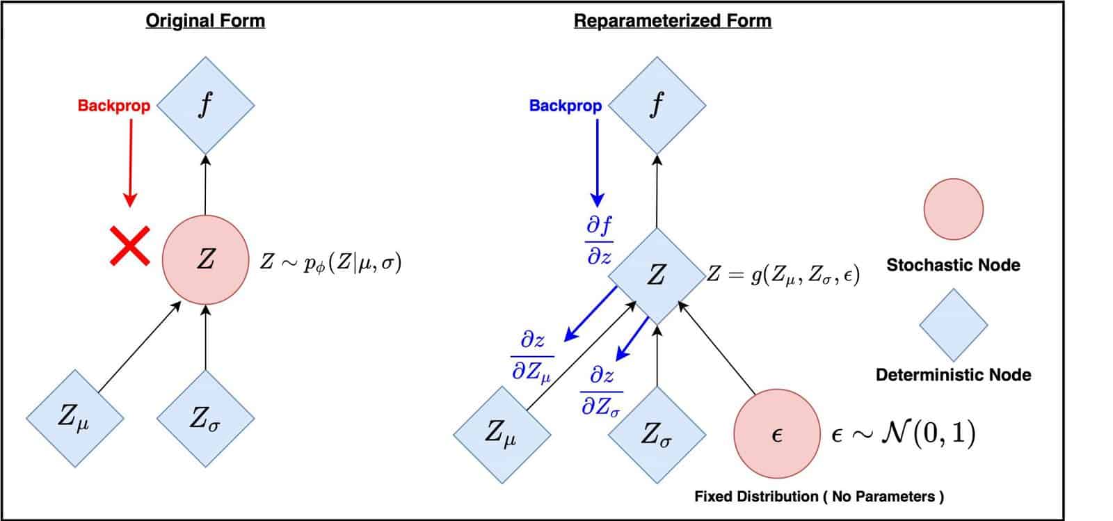
This is where the reparameterization trick comes into play. It helps avoid the problem by transforming the random node in the latent space into a deterministic counterpart. Doing so ensures that gradients can propagate seamlessly through the network (Figure 3), facilitating effective training. The essence of the trick lies in introducing an auxiliary random variable, typically drawn from a standard normal distribution.

Mathematically, this can be represented as:

Here, is sampled from a standard normal distribution, that is, . The symbol stands for element-wise multiplication.

By adopting this approach, the VAE can harness the benefits of randomness in the latent space while still maintaining the tractability of training. This balance is crucial for the VAE’s dual objectives of accurate reconstructions and effective generation.

Having delved deep into the theoretical underpinnings of VAE, it’s time to bring that knowledge to life. We’ll embark on a comprehensive code walkthrough in the next segment, demystifying each component step-by-step. Following that, we’ll dive into some exciting experiments, showcasing the prowess of our trained VAE in action. Let’s transition from theory to hands-on practice!

---

Configuring Your Development Environment

To follow this guide, you need to have the torch, torchvision, and matplotlib libraries installed on your system.

Luckily, all these libraries are pip-installable:

$ pip install torch>=2.0.1
$ pip install torchvision>=0.15.2
$ pip install matplotlib==3.7.2

---

Need Help Configuring Your Development Environment?

All that said, are you:

• Short on time?
• Learning on your employer’s administratively locked system?
• Wanting to skip the hassle of fighting with the command line, package managers, and virtual environments?
• Ready to run the code immediately on your Windows, macOS, or Linux system?

Then join PyImageSearch University today!

Gain access to Jupyter Notebooks for this tutorial and other PyImageSearch guides pre-configured to run on Google Colab’s ecosystem right in your web browser! No installation required.

And best of all, these Jupyter Notebooks will run on Windows, macOS, and Linux!

---

Project Structure

We first need to review our project directory structure.

Start by accessing this tutorial’s “Downloads” section to retrieve the source code and example images.

From there, take a look at the directory structure:

$ tree -L 2
.
├── output
│   ├── embedding_visualize.png
│   ├── image_grid_on_embeddings.png
│   ├── latent_distribution.png
│   ├── linearly_sampled_reconstructions.png
│   ├── model_weights
│   ├── normally_sampled_reconstructions.png
│   ├── real_test_images_after_train.png
│   ├── real_test_images_before_train.png
│   ├── reconstruct_after_train.png
│   ├── reconstruct_before_train.png
│   └── training_progress
├── pyimagesearch
│   ├── __init__.py
│   ├── config.py
│   ├── network.py
│   └── utils.py
├── test.py
└── train.py

5 directories, 15 files

In the pyimagesearch directory, we have the following files:

• config.py: This configuration file is for training the variational autoencoder.
• utils.py: This file contains utilities like the loss function of VAE, post-training analysis, and a validation method for evaluating the VAE during training.
• network.py: Contains the VAE architecture implementation in PyTorch.

In the core directory, we have the following:

• train.py: The script for training the VAE on the Fashion-MNIST dataset.
• test.py: The script for evaluating the trained VAE on the test dataset and conducting post-training analysis.
• output: This folder hosts the model weights, training reconstruction progress over each epoch, evaluation of the test set, and post-training analysis of the VAE.

---

About the Dataset

In this tutorial, we employ the Fashion-MNIST dataset for training our variational autoencoder model.

---

Overview

Fashion-MNIST is a dataset of Zalando’s article images consisting of the following:

• training set of 60,000 examples
• test set of 10,000 examples

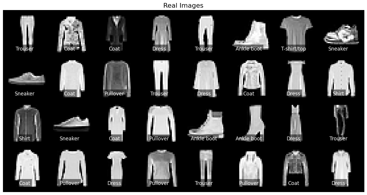
Each sample is a 28x28 grayscale image associated with a label from 10 classes (Figure 5). It serves as a direct drop-in replacement for the original Fashion-MNIST dataset for benchmarking machine learning algorithms, with the benefit of being more representative of the actual data tasks and challenges.

---

Class Distribution

The Fashion-MNIST dataset is balanced, which means it has an equal number of samples from each class. The 10 classes are T-shirt/top, Trouser, Pullover, Dress, Coat, Sandal, Shirt, Sneaker, Bag, and Ankle boot. Each class has 6,000 images in the training set and 1,000 in the test set.

---

Data Preprocessing

Before training the autoencoder, the images from the dataset are preprocessed. Each image in the dataset is a 28x28 grayscale image. The pixel values fall from 0 to 255. As a preprocessing step, these pixel values are normalized to fall from 0 to 1. This is achieved by dividing each pixel value by 255. This normalization helps in faster and more stable convergence during training.

---

Data Split

The dataset is split into two parts: a training set and a test set. The training set, which contains 60,000 images, is used to train the autoencoder, and the test set, which includes 10,000 images, is used to evaluate the model’s performance. It is essential to separate the data used for training from the data used for testing to get an unbiased measure of the model’s performance.

---

Configuring the Prerequisites

Before we start our implementation, let’s review our project’s configuration. For that, we will move on to the config.py script located in the pyimagesearch directory.

The config.py script sets up the autoencoder model hyperparameters and creates an output directory for storing training progress metadata, model weights, and post-training analysis plots. It also defines the class labels dictionary mapping from integer to human-readable format.

# import the necessary packages
import os

import torch

# set device to 'cuda' if CUDA is available, 'mps' if MPS is available,
# or 'cpu' otherwise for model training and testing
DEVICE = (
    "cuda"
    if torch.cuda.is_available()
    else "mps"
    if torch.backends.mps.is_available()
    else "cpu"
)

# define model hyperparameters
LR = 0.001
PATIENCE = 2
IMAGE_SIZE = 32
CHANNELS = 1
BATCH_SIZE = 64
EMBEDDING_DIM = 2
EPOCHS = 100
SHAPE_BEFORE_FLATTENING = (128, IMAGE_SIZE // 8, IMAGE_SIZE // 8)

# create output directory
output_dir = "output"
os.makedirs("output", exist_ok=True)

Lines 2-4 import the os module, which provides functionality for operating system-dependent operations, and the torch module to determine the available computational device (CUDA GPU, MPS, or CPU) for model training and inference.

From Lines 8-14, we set the DEVICE variable based on the available hardware. If CUDA (used for NVIDIA GPUs) is available, DEVICE is set to cuda. If CUDA isn’t available but MPS (Metal Performance Shaders, used for Apple devices) is available, DEVICE is set to “mps”. If neither CUDA nor MPS is available, DEVICE defaults to cpu.

Then, from Lines 17-24, we define various hyperparameters and settings for the model:

• LR: Learning rate for the optimizer.
• PATIENCE: Used for reducing the learning rate, indicating how many epochs to wait for before reducing the learning rate.
• IMAGE_SIZE: The size (height and width) of the input images.
• CHANNELS: Number of channels in the input image (1 for grayscale, 3 for RGB).
• BATCH_SIZE: Number of samples processed before the model is updated.
• EMBEDDING_DIM: Dimensionality of the embedding space (for a latent space in a VAE model).
• EPOCHS: Total number of training epochs.
• SHAPE_BEFORE_FLATTENING: The shape of the tensor before it’s flattened, used in the decoder of VAE for reshaping the latent space from a vector to a tensor.

On Lines 27 and 28, an output directory is created where the results from the model (e.g., saved model weights or performance plots) are stored.

# create the training_progress directory inside the output directory
training_progress_dir = os.path.join(output_dir, "training_progress")
os.makedirs(training_progress_dir, exist_ok=True)

# create the model_weights directory inside the output directory
# for storing variational autoencoder weights
model_weights_dir = os.path.join(output_dir, "model_weights")
os.makedirs(model_weights_dir, exist_ok=True)

# define model_weights, reconstruction & real before training images paths
MODEL_WEIGHTS_PATH = os.path.join(model_weights_dir, "best_vae.pt")

On Lines 31 and 32, we create training_progress_dir, which would store the reconstruction output of a variational autoencoder during training for each epoch.

Next, we create a model_weights_dir, which hosts the best variational autoencoder weights (Lines 36-40).

FILE_RECON_BEFORE_TRAINING = os.path.join(
    output_dir, "reconstruct_before_train.png"
)
FILE_REAL_BEFORE_TRAINING = os.path.join(
    output_dir, "real_test_images_before_train.png"
)

# define reconstruction & real after training images paths
FILE_RECON_AFTER_TRAINING = os.path.join(
    output_dir, "reconstruct_after_train.png"
)
FILE_REAL_AFTER_TRAINING = os.path.join(
    output_dir, "real_test_images_after_train.png"
)

# define latent space and image grid embeddings plot paths
LATENT_SPACE_PLOT = os.path.join(output_dir, "embedding_visualize.png")
IMAGE_GRID_EMBEDDINGS_PLOT = os.path.join(
    output_dir, "image_grid_on_embeddings.png"
)

# define linearly and normally sampled latent space reconstructions plot paths
LINEARLY_SAMPLED_RECONSTRUCTIONS_PLOT = os.path.join(
    output_dir, "linearly_sampled_reconstructions.png"
)
NORMALLY_SAMPLED_RECONSTRUCTIONS_PLOT = os.path.join(
    output_dir, "normally_sampled_reconstructions.png"
)

# define class labels dictionary
CLASS_LABELS = {
    0: "T-shirt/top",
    1: "Trouser",
    2: "Pullover",
    3: "Dress",
    4: "Coat",
    5: "Sandal",
    6: "Shirt",
    7: "Sneaker",
    8: "Bag",
    9: "Ankle boot",
}

Lines 41-54 define paths where images will be saved before and after training the model. The images (or plots) are reconstructions from an untrained and trained model along with the corresponding real images.

Next, we define some post-training analysis plot paths for storing visualization results such as LATENT_SPACE_PLOT, IMAGE_GRID_EMBEDDINGS_PLOT, LINEARLY_SAMPLED_RECONSTRUCTIONS_PLOT, and NORMALLY_SAMPLED_RECONSTRUCTIONS_PLOT on Lines 57-68.

Lastly, we establish a CLASS_LABELS dictionary on Lines 71-82. This assists in assessing the quality of the reconstruction and determining the class to which the reconstruction pertains, as we possess both test images and labels for that specific reconstruction.

---

Defining the Utilities

Now that the configuration has been defined, we can determine the utilities for validating the autoencoder during training and post-training analysis plots.

If you’ve followed along with the previous lesson in this series, you may recall our deep dive into various utilities designed to aid in the training and analysis of deep learning models. In the context of this autoencoder tutorial, I’ve prepared a utils.py script that arms you with functions for tasks such as random image extraction, image visualization, and latent space plotting, to name a few.

Here’s a brief rundown:

• Image Visualization: extract_random_images, display_images, and display_random_images collectively handle the extraction and display of random images from our dataset.
• Autoencoder Validation: The validate function is instrumental in monitoring our autoencoder’s performance at the end of each training epoch.
• Latent Space Analysis: The real magic of autoencoders lies in their ability to represent complex data in a reduced-dimensional space. Functions like get_test_embeddings, plot_latent_space, get_random_test_images_embeddings, and plot_image_grid_on_embeddings are designed specifically for this purpose, allowing you to visualize and interpret the latent embeddings of your trained model.

While we won’t delve into the specifics here (as they were thoroughly explored in the previous lesson of this series), rest assured these utilities are pivotal in fine-tuning, validating, and analyzing our autoencoder model.

However, in this lesson, we do emphasize the VAE loss function, a critical component of our utilities. This loss function, composed of the KL divergence and reconstruction loss, is pivotal for optimizing the VAE architecture.

import torch
import torch.nn as nn

We start by importing torch and torch.nn on Lines 6 and 7. The torch.nn is a sub-library in PyTorch containing neural network layers, loss functions, and utilities.

def vae_gaussian_kl_loss(mu, logvar):
    # see Appendix B from VAE paper:
    # Kingma and Welling. Auto-Encoding Variational Bayes. ICLR, 2014
    # https://arxiv.org/abs/1312.6114
    KLD = -0.5 * torch.sum(1 + logvar - mu.pow(2) - logvar.exp(), dim=1)
    return KLD.mean()


def reconstruction_loss(x_reconstructed, x):
    bce_loss = nn.BCELoss()
    return bce_loss(x_reconstructed, x)


def vae_loss(y_pred, y_true):
    mu, logvar, recon_x = y_pred
    recon_loss = reconstruction_loss(recon_x, y_true)
    kld_loss = vae_gaussian_kl_loss(mu, logvar)
    return 500 * recon_loss + kld_loss

Lines 382-387 compute the Kullback-Leibler Divergence (KLD) between the learned latent variable distribution and a standard normal distribution. The formula is derived from the VAE paper. mu and logvar are the mean and log variance outputs from the encoder part of the VAE.

Next, on Lines 390-392, we compute the Binary Cross-Entropy (BCE) loss between the original input x and its reconstruction x_reconstructed. This loss measures how well the VAE has reconstructed the input data.

Finally, we compute the total loss for training the VAE by combining the reconstruction loss and the KL divergence loss on Lines 395-399. The reconstruction loss is scaled by a factor of 500. This weighting factor balances the two components of the loss. Adjusting this factor can influence the trade-off between the fidelity of the reconstructions and the regularity of the latent space.

---

Defining the Network

# import the necessary libraries
import torch
import torch.nn as nn
import torch.nn.functional as F
from torch.distributions.normal import Normal

We start by importing the required packages: torch, torch.nn, torch.nn.functional, and torch.distributions.normal on Lines 1-5.

The torch.nn.functional module contains functions that operate on tensors and are used in building neural networks. Unlike torch.nn, which provides classes, torch.nn.functional provides functions. This is useful for operations that don’t have any parameters (e.g., activation functions, certain loss functions, and, in our case, using it for the ReLU activation function).

We import the Normal class from torch.distributions, which provides functionalities to create and manipulate normal (Gaussian) distributions. We use it in the Sampling class to sample a tensor from a normal distribution.

# define a class for sampling
# this class will be used in the encoder for sampling in the latent space
class Sampling(nn.Module):
    def forward(self, z_mean, z_log_var):
        # get the shape of the tensor for the mean and log variance
        batch, dim = z_mean.shape
        # generate a normal random tensor (epsilon) with the same shape as z_mean
        # this tensor will be used for reparameterization trick
        epsilon = Normal(0, 1).sample((batch, dim)).to(z_mean.device)
        # apply the reparameterization trick to generate the samples in the
        # latent space
        return z_mean + torch.exp(0.5 * z_log_var) * epsilon

Next, we define a Sampling class that provides a mechanism to sample from the latent space of a VAE using the reparameterization trick, which allows for gradient-based optimization during training.

On Line 10, we define the Sampling class as a subclass of nn.Module that allows us to use it as part of a larger neural network model.

Then, the forward method defines the forward pass of the module on Line 11. In PyTorch, it internally invokes the forward method when you call an nn.Module object. Here, the method takes two arguments: z_mean and z_log_var, which represent the mean and log variance of the latent variable’s distribution, respectively.

On Lines 13 and 16, the shape of the z_mean tensor is extracted to get the batch size and the dimension of the latent space. A random tensor epsilon is sampled from a standard normal distribution (mean 0 and variance 1) with the same shape as z_mean. This tensor is used for the reparameterization trick. The .to(z_mean.device) ensures the epsilon tensor is on the same device (CPU or GPU) as the z_mean tensor.

Finally, on Line 19, we apply the reparameterization trick and return it to the calling function. Instead of sampling from the distribution parameterized by z_mean and z_log_var directly, the trick introduces an auxiliary random variable epsilon and a deterministic transformation.

• The term torch.exp(0.5 * z_log_var) computes the standard deviation (since the input is the log variance).
• The sampled latent variable is then computed as the mean plus the standard deviation multiplied by the random tensor epsilon.

# define the encoder
class Encoder(nn.Module):
    def __init__(self, image_size, embedding_dim):
        super(Encoder, self).__init__()
        # define the convolutional layers for downsampling and feature
        # extraction
        self.conv1 = nn.Conv2d(1, 32, 3, stride=2, padding=1)
        self.conv2 = nn.Conv2d(32, 64, 3, stride=2, padding=1)
        self.conv3 = nn.Conv2d(64, 128, 3, stride=2, padding=1)
        # define a flatten layer to flatten the tensor before feeding it into
        # the fully connected layer
        self.flatten = nn.Flatten()
        # define fully connected layers to transform the tensor into the desired
        # embedding dimensions
        self.fc_mean = nn.Linear(
            128 * (image_size // 8) * (image_size // 8), embedding_dim
        )
        self.fc_log_var = nn.Linear(
            128 * (image_size // 8) * (image_size // 8), embedding_dim
        )
        # initialize the sampling layer
        self.sampling = Sampling()

    def forward(self, x):
        # apply convolutional layers with relu activation function
        x = F.relu(self.conv1(x))
        x = F.relu(self.conv2(x))
        x = F.relu(self.conv3(x))
        # flatten the tensor
        x = self.flatten(x)
        # get the mean and log variance of the latent space distribution
        z_mean = self.fc_mean(x)
        z_log_var = self.fc_log_var(x)
        # sample a latent vector using the reparameterization trick
        z = self.sampling(z_mean, z_log_var)
        return z_mean, z_log_var, z

Next, we define the encoder part of a VAE, consisting of convolutional layers for feature extraction, fully connected layers for transforming features into latent space parameters, and a sampling mechanism to generate latent vectors.

On Line 23, we define the class Encoder as a subclass of PyTorch’s nn.Module.

The __init__ method initializes the encoder with the necessary layers from Lines 24-43. It takes two parameters: image_size, representing the size of the input images, and embedding_dim, representing the dimensionality of the latent space. Below are the layers the encoder comprises of:

• Convolutional Layers: Three convolutional layers are defined for downsampling and feature extraction. They progressively increase the number of channels and reduce the spatial dimensions of the input.
• Flatten Layer: A flatten layer is defined to convert the 3D tensor output from the convolutional layers into a 1D tensor.
• Fully Connected Layers: Two fully connected layers are defined to transform the flattened tensor into the mean and log variance of the latent space distribution.
• Sampling Layer: An instance of the previously defined Sampling class is created to handle the reparameterization trick.

From Lines 45-57, the forward method defines the forward pass of the encoder. It takes an input tensor x (representing a batch of images) and returns three outputs: z_mean, z_log_var, and z.

A call to the following layers, along with necessary activation functions, is made:

• Convolutional Layers with ReLU Activation: The input is passed through the three convolutional layers, each followed by a ReLU activation function.
• Flattening: The 3D tensor is flattened into a 1D tensor.
• Mean and Log Variance: The flattened tensor is passed through the fully connected layers to obtain the mean (z_mean) and log variance (z_log_var) of the latent space distribution.
• Sampling: The Sampling layer is called with z_mean and z_log_var to sample a latent vector z using the reparameterization trick.

# define the decoder
class Decoder(nn.Module):
    def __init__(self, embedding_dim, shape_before_flattening):
        super(Decoder, self).__init__()
        # define a fully connected layer to transform the latent vector back to
        # the shape before flattening
        self.fc = nn.Linear(
            embedding_dim,
            shape_before_flattening[0]
            * shape_before_flattening[1]
            * shape_before_flattening[2],
        )
        # define a reshape function to reshape the tensor back to its original
        # shape
        self.reshape = lambda x: x.view(-1, *shape_before_flattening)
        # define the transposed convolutional layers for the decoder to upsample
        # and generate the reconstructed image
        self.deconv1 = nn.ConvTranspose2d(
            128, 64, 3, stride=2, padding=1, output_padding=1
        )
        self.deconv2 = nn.ConvTranspose2d(
            64, 32, 3, stride=2, padding=1, output_padding=1
        )
        self.deconv3 = nn.ConvTranspose2d(
            32, 1, 3, stride=2, padding=1, output_padding=1
        )

    def forward(self, x):
        # pass the latent vector through the fully connected layer
        x = self.fc(x)
        # reshape the tensor
        x = self.reshape(x)
        # apply transposed convolutional layers with relu activation function
        x = F.relu(self.deconv1(x))
        x = F.relu(self.deconv2(x))
        # apply the final transposed convolutional layer with a sigmoid
        # activation to generate the final output
        x = torch.sigmoid(self.deconv3(x))
        return x

On Line 61, we define the Decoder class, which like Encoder, inherits from the nn.Module class. The decoder of a variational autoencoder performs the opposite of the encoder, taking the latent space as input and generating an image at the output.

The __init__ method initializes the decoder with the necessary layers from Lines 62-85. It takes two parameters: embedding_dim (represents the dimensionality of the latent space) and shape_before_flattening (is the tensor’s shape before it was flattened in the encoder). The decoder comprises of following layers and functionalities in the __init__ method:

• Fully Connected Layer: The self.fc layer transforms the latent vector back to the tensor’s shape before it was flattened in the encoder.
• Reshape Function: The self.reshape lambda function reshapes the tensor back to its original 3D shape after passing through the fully connected layer.
• Transposed Convolutional Layers: Three transposed convolutional layers (deconv1, deconv2, deconv3) are defined to upsample the tensor and generate the reconstructed image.

On Lines 87-98, the forward method defines the forward pass of the decoder. It takes a latent vector x as input and returns the reconstructed image. During this forward pass, calls to the following layers and functions are made:

• Fully Connected Layer: The latent vector is passed through the fully connected layer to expand its dimensions.
• Reshaping: The tensor is reshaped to its original 3D shape using the self.reshape function.
• Transposed Convolutional Layers with ReLU Activation: The tensor is passed through two transposed convolutional layers (deconv1 and deconv2), each followed by a ReLU activation function.
• Final Transposed Convolutional Layer with Sigmoid Activation: The tensor is passed through the final transposed convolutional layer (deconv3) and then through a sigmoid activation function. The sigmoid activation ensures that the output values are between 0 and 1, which is suitable for image pixel values.

# define the vae class
class VAE(nn.Module):
    def __init__(self, encoder, decoder):
        super(VAE, self).__init__()
        # initialize the encoder and decoder
        self.encoder = encoder
        self.decoder = decoder

    def forward(self, x):
        # pass the input through the encoder to get the latent vector
        z_mean, z_log_var, z = self.encoder(x)
        # pass the latent vector through the decoder to get the reconstructed
        # image
        reconstruction = self.decoder(z)
        # return the mean, log variance and the reconstructed image
        return z_mean, z_log_var, reconstruction

Finally, with the Encoder and Decoder classes defined, we combine them into a unified VAE class.

The __init__ method initializes the VAE with the provided encoder and decoder from Lines 103-107. The encoder and decoder are passed as arguments when creating an instance of the VAE class. The provided encoder and decoder are assigned to self.encoder and self.decoder, respectively. These will be used in the forward pass.

On Lines 109-116, the forward method defines the forward pass of the VAE. It takes an input tensor x (representing a batch of images) and returns three outputs: z_mean, z_log_var, and reconstruction.

• Encoder: The input x is passed through the encoder, which returns the mean (z_mean), log variance (z_log_var), and a sample (z) from the latent space distribution.
• Decoder: The sampled latent vector z is then passed through the decoder to produce the reconstructed image (reconstruction).

---

Training the Variational Autoencoder

In this section, we set up and train a VAE on the Fashion-MNIST dataset. First, we preprocess the data, initialize the model, optimizer, and scheduler, and then train the model for a specified number of epochs, saving the best model based on validation loss.

# USAGE
# python train.py

# import the necessary packages
from pyimagesearch import config, network, utils
from torchvision import datasets, transforms
import torch.optim as optim
import torch
import os

import matplotlib

# change the backend based on the non-gui backend available
matplotlib.use("agg")

We start by importing the necessary modules and functions from the pyimagesearch package, torchvision, torch, and optim from Lines 5-11.

Line 14 sets the backend of Matplotlib to “agg”, which is a non-GUI backend suitable for scripts and web servers.

# define the transformation to be applied to the data
transform = transforms.Compose(
    [transforms.Pad(padding=2), transforms.ToTensor()]
)

# load the FashionMNIST training data and create a dataloader
trainset = datasets.FashionMNIST(
    "data", train=True, download=True, transform=transform
)
train_loader = torch.utils.data.DataLoader(
    trainset, batch_size=config.BATCH_SIZE, shuffle=True
)

# load the FashionMNIST test data and create a dataloader
testset = datasets.FashionMNIST(
    "data", train=False, download=True, transform=transform
)
test_loader = torch.utils.data.DataLoader(
    testset, batch_size=config.BATCH_SIZE, shuffle=True
)

Lines 18-20 define a transformation pipeline to preprocess the images. Images are padded by 2 pixels and then converted to tensors.

Then, from Lines 23-36,

• The Fashion-MNIST training and test datasets are loaded using datasets.FashionMNIST.
• The data is transformed using the previously defined transformations.
• DataLoaders for both training and test datasets are created. These will be used to iterate over the datasets in batches.

# instantiate the encoder and decoder models
encoder = network.Encoder(config.IMAGE_SIZE, config.EMBEDDING_DIM).to(
    config.DEVICE
)
decoder = network.Decoder(
    config.EMBEDDING_DIM, config.SHAPE_BEFORE_FLATTENING
).to(config.DEVICE)
# pass the encoder and decoder to VAE class
vae = network.VAE(encoder, decoder)

In the above lines,

• Instances of the encoder and decoder are created using configurations from the config module.
• These instances are then passed to the VAE class to create the VAE model.

# instantiate optimizer and scheduler
optimizer = optim.Adam(
    list(encoder.parameters()) + list(decoder.parameters()), lr=config.LR
)
scheduler = torch.optim.lr_scheduler.ReduceLROnPlateau(
    optimizer, mode="min", factor=0.1, patience=config.PATIENCE, verbose=True
)

The Adam optimizer is initialized with the parameters of both the encoder and decoder on Lines 49-51.

A learning rate scheduler is also initialized to reduce the learning rate when the validation loss plateaus (Lines 52-54).

# initialize the best validation loss as infinity
best_val_loss = float("inf")

# start training by looping over the number of epochs
for epoch in range(config.EPOCHS):
    # set the vae model to train mode
    # and move it to CPU/GPU
    vae.train()
    vae.to(config.DEVICE)

    running_loss = 0.0
    # loop over the batches of the training dataset
    for batch_idx, (data, _) in enumerate(train_loader):
        data = data.to(config.DEVICE)
        optimizer.zero_grad()

        # forward pass through the VAE
        pred = vae(data)

        # compute the VAE loss
        loss = utils.vae_loss(pred, data)

        # backward pass and optimizer step
        loss.backward()
        optimizer.step()

        running_loss += loss.item()

Now starts the training loop for variational autoencoder for a specified number of epochs (from the config module).

Within each epoch:

• The VAE model is set to training mode and moved to the appropriate device (CPU/GPU).
• The training dataset is iterated over in batches.
• For each batch, the data is passed through the VAE, and the loss is computed using the utils.vae_loss function.
• Gradients are backpropagated, and the optimizer updates the model parameters.
• The training loss is accumulated.

    # compute average loss for the epoch
    train_loss = running_loss / len(train_loader)
    # compute validation loss for the epoch
    val_loss = utils.validate(vae, test_loader)
    # print training and validation loss at every 20 epochs
    if epoch % 20 == 0 or (epoch+1) == config.EPOCHS:
        print(
            f"Epoch {epoch} | Train Loss: {train_loss:.4f} | Val Loss: {val_loss:.4f}"
        )

    # save best vae model weights based on validation loss
    if val_loss < best_val_loss:
        best_val_loss = val_loss
        torch.save(
            {"vae": vae.state_dict()},
            config.MODEL_WEIGHTS_PATH,
        )
    # adjust learning rate based on the validation loss
    scheduler.step(val_loss)

Continuing the training loop:

• After processing all batches, the average training loss for the epoch is computed.
• The model is then validated on the test dataset, and the validation loss is computed.
• Every 20 epochs, or on the last epoch, the training and validation losses are printed.
• If the current epoch’s validation loss is the best so far, the model’s weights are saved.
• The learning rate scheduler adjusts the learning rate based on the validation loss.

With that, we’ve completed the training of a variational autoencoder on the Fashion-MNIST dataset. In the following section, we’ll examine the performance of the variational autoencoder under various testing scenarios.

---

Post-Training Analysis of Variational Autoencoder

After training our Variational Autoencoder (VAE) on the Fashion-MNIST dataset, it’s essential to dive into its performance metrics and truly understand what it has achieved. This post-training exploration gives us a clear picture of the VAE’s ability to encode images, navigate the latent space, and produce outputs that strike a balance between originality and familiarity.

Our deep dive into these evaluations not only stands as a testament to the VAE’s capabilities but also showcases its wide-ranging applications. From refining existing images to creating entirely new visuals, the possibilities are vast.

Here’s a closer look at the experiments we conducted:

• Evaluating the VAE’s image reconstructions after training.
• Comparing the latent space distribution of a Convolutional Autoencoder from a previous blog post with our VAE.
• A detailed visualization of the latent space of the trained VAE.
• Generating a series of images linearly spaced on the VAE’s embeddings.
• Visualizing reconstructions from points linearly sampled within the latent space.

---

Reconstruction by Variational Autoencoder After Training

After training our VAE, it’s essential to gauge its reconstruction capabilities. By feeding it a set of validation images and comparing the outputs with the originals, we can determine how effectively the VAE has captured the essence of the dataset. As shown in Figure 6, the generated images appear quite realistic and closely resemble the original data, showcasing the VAE’s ability to replicate visual patterns with minimal loss of detail.

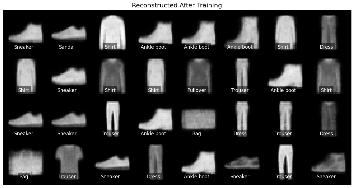
Furthermore, there’s a diverse representation across classes, ensuring distinct visual differences between categories, such as between sneakers and ankle boots. This diversity in reconstructions also indicates that our VAE doesn’t suffer from mode collapse, a common issue where generative models produce similar outputs for different classes.

---

Visualize the Distribution of the Latent Space of Trained Convolutional Autoencoder vs. Variational Autoencoder

In a previous blog post, we explored the Convolutional Autoencoder (CAE). When comparing its latent space with those of our VAEs, distinct differences emerge. As shown in Figure 7, the CA’s latent space doesn’t closely follow a normal distribution, whereas the VAE’s latent space (Figure 8) aligns well with it and is centered around 0.

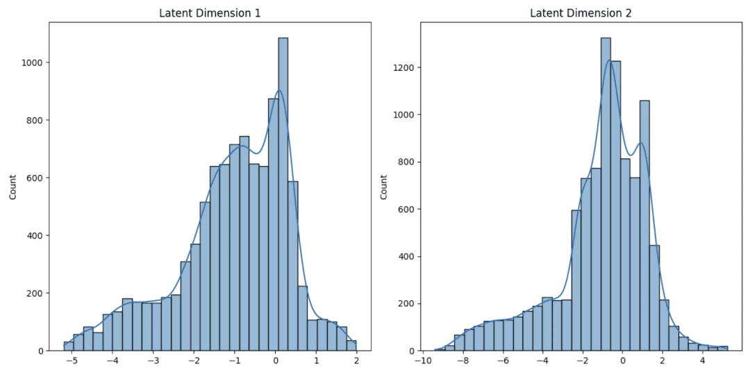
This normal distribution in the VAE’s latent space ensures a more continuous and dense representation, which often leads to better and more consistent image generation. Both models aim to capture the data’s underlying structure, but their methods and outcomes vary. This comparison deepens our understanding of each generative model’s unique characteristics and strengths.

---

Latent Space Plot of Trained Variational Autoencoder

The latent space of our VAE is a treasure trove of information. By visualizing this space, colored by clothing type, as shown in Figure 9, we can discern clusters, patterns, and potential correlations between different attributes. Each point in this space represents a condensed version of an image, and its location provides insights into the image’s features.

Similar class labels tend to form clusters, as observed with the Convolutional Autoencoder. This clustering remains consistent despite the VAE incorporating both the KL divergence loss and the reconstruction loss. The KL term encourages the latent space to follow a standard normal distribution centered around 0. As a result, most of the latent values tend to lie within a range close to -3 to 3, based on the properties of the standard normal distribution.

Notably, the labels were not used during training; the VAE independently learned the various forms of clothing to minimize reconstruction loss. Exploring this space offers a deeper understanding of the VAE’s internal mechanics and the relationships it has inferred among the dataset images.

---

Linearly Separated Images (Grid) on Embeddings of Trained Variational Autoencoder

In our previous tutorial on Convolutional Autoencoders (CAEs), we observed certain limitations in the latent space. Notably, there were regions where the encoded images were sparse, leading to voids. These voids posed challenges when generating new images, as points sampled from these areas often resulted in poorly formed or unrecognizable outputs. Additionally, the distribution of points in the CAE’s latent space was undefined, making it challenging to determine where to sample from.

Fast forward to our experiments with the Variational Autoencoder (VAE), the landscape of the latent space appears markedly different. One of the defining characteristics of VAEs is their ability to enforce a continuous latent space, primarily due to the KL divergence term in their loss function. This continuity ensures that almost any point sampled from this space can be decoded into a meaningful image.

Comparing our VAE results with the CAE findings, we notice a significant reduction in the voids or “empty spaces” in the latent space, as shown in Figure 10. Images generated from the VAE’s latent space exhibit a higher degree of coherence and quality. Even when we linearly sample points between two images, the VAE produces a smooth transition, capturing the nuances of each intermediate step. This is in stark contrast to the CAE, where linear sampling could lead to abrupt or unrecognizable transitions.

Furthermore, the VAE’s latent space is centered around zero and follows a normal distribution, providing a clear guideline for sampling. This structured approach to the latent space alleviates the challenges we faced with the CAE, where any point on the 2D plane could technically be a valid choice, but with no guarantee of a meaningful output.

In essence, the VAE addresses many of the challenges we identified with the CAE. Its ability to maintain a continuous and structured latent space makes it a powerful tool for generating diverse and high-quality images, bridging the gaps we observed in our previous experiments with the CAE.

---

Reconstructions by the Trained Decoder of Variational Autoencoder Using the Points Sampled from Normal Distribution

A hallmark of the VAE is its ability to generate novel images by sampling points from a standard normal distribution and decoding them. This process taps into the VAE’s trained decoder to produce images that, while not explicitly present in the Fashion-MNIST dataset, are constructed using the learned features and patterns. From generating t-shirts and trousers to sandals and slippers, the VAE captures a wide range of fashion items.

Figure 11 provides a glimpse into the VAE’s generative prowess. Showcasing its capacity to create diverse and realistic fashion item reconstructions from random points in the latent space, the VAE covers the entire spectrum of the Fashion-MNIST dataset, capturing the essence of the fashion world in a truly remarkable manner.

---

---

Summary

This tutorial offers a deep dive into the world of Variational Autoencoders (VAEs), beginning with a foundational understanding of their structure, including the roles of the encoder and decoder. We contrast the traditional Convolutional Autoencoder (CAE) with the VAE, emphasizing the significance of the Gaussian distribution in the latter. The tutorial further elaborates on the VAE’s objective function, highlighting the balance between reconstruction loss and KL divergence and introduces the reparameterization trick, a crucial component for training VAEs.

Our dataset of choice is the Fashion-MNIST, a popular collection of fashion items. We explore its structure, class distribution, and the necessary preprocessing steps to make it suitable for training. The partitioning of this dataset into training and validation subsets is also detailed.

As we delve into the implementation, we discuss the configuration prerequisites, the creation of essential utilities, and the architecture of the VAE network.

The core of this tutorial revolves around the training process of the VAE, where we meticulously guide readers through each step. Once trained, we transition into a comprehensive post-training analysis. This section showcases a series of experiments, from evaluating the VAE’s image reconstructions to comparing the latent space distributions of a previously trained Convolutional Autoencoder and our VAE. We also visualize the latent space, generate images based on linearly spaced embeddings, and demonstrate the VAE’s ability to reconstruct images from points sampled from a normal distribution.

By the tutorial’s conclusion, readers will possess a robust understanding of VAEs, appreciating their capabilities in image generation, reconstruction, and the nuances of working with the Fashion-MNIST dataset.

In our upcoming tutorial, we’ll explore the CelebA dataset with Variational Autoencoders (VAEs), focusing on its architecture, training nuances, and post-training experiments. We’ll delve into image reconstruction, latent space arithmetic, and the unique capabilities of VAEs in generative modeling. Stay tuned for a deeper dive into VAEs and their applications.

---

Citation Information

Sharma, A. “A Deep Dive into Variational Autoencoders with PyTorch,” PyImageSearch, P. Chugh, A. R. Gosthipaty, S. Huot, K. Kidriavsteva, and R. Raha, eds., 2023, https://pyimg.co/7e4if

@incollection{Sharma_2023_VAE,
  author = {Aditya Sharma},
  title = {A Deep Dive into Variational Autoencoders with {PyTorch}},
  booktitle = {PyImageSearch},
  editor = {Puneet Chugh and Aritra Roy Gosthipaty and Susan Huot and Kseniia Kidriavsteva and Ritwik Raha},
  year = {2023},
  url = {https://pyimg.co/7e4if},
}

---

---

To download the source code to this post (and be notified when future tutorials are published here on PyImageSearch), simply enter your email address in the form below!

The post A Deep Dive into Variational Autoencoders with PyTorch appeared first on PyImageSearch.

Find A Teacher Form:
https://docs.google.com/forms/d/1vREBnX5n262umf4wU5U2pyTwvk9O-JrAgblA-wH9GFQ/viewform?edit_requested=true#responses

Email:
public1989two@gmail.com






www.itsec.hk
www.itsec.vip
www.itseceu.uk